
![]()


Citation
Zuguang Gu, et al., cola: an R/Bioconductor package for consensus partitioning through a general framework, Nucleic Acids Research, 2021. https://doi.org/10.1093/nar/gkaa1146
Zuguang Gu, et al., Improve consensus partitioning via a hierarchical procedure. Briefings in bioinformatics 2022. https://doi.org/10.1093/bib/bbac048
Install
cola is available on Bioconductor, you can install it by:
if (!requireNamespace("BiocManager", quietly = TRUE))
    install.packages("BiocManager")
BiocManager::install("cola")
The latest version can be installed directly from GitHub:
library(devtools)
install_github("jokergoo/cola")
Methods
The cola supports two types of consensus partitioning.
Standard consensus partitioning
Features
- It modularizes the consensus clustering processes that various methods can be easily integrated in different steps of the analysis.
- It provides rich visualizations for intepreting the results.
- It allows running multiple methods at the same time and provides functionalities to compare results in a straightforward way.
- It provides a new method to extract features which are more efficient to separate subgroups.
- It generates detailed HTML reports for the complete analysis.
Workflow
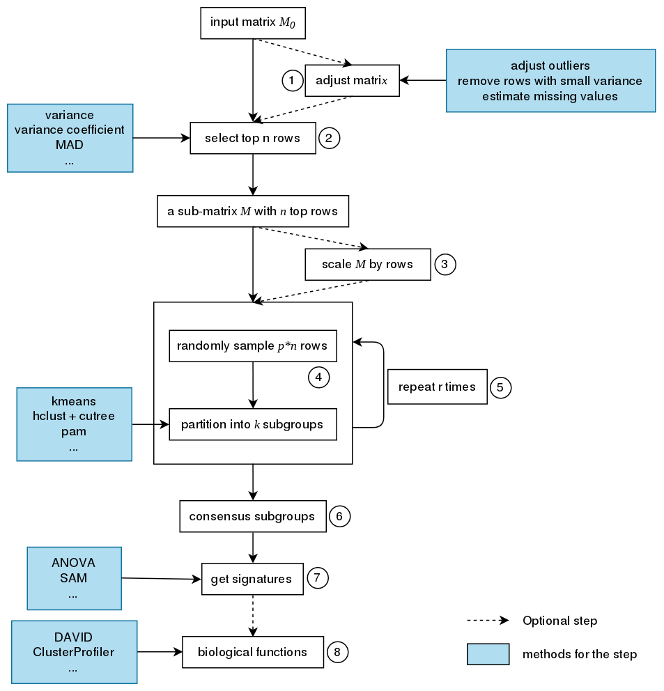
The steps of consensus partitioning is:
- Clean the input matrix. The processing are: adjusting outliers, imputing missing values and removing rows with very small variance. This step is optional.
- Extract subset of rows with highest scores. Here “scores” are calculated by a certain method. For gene expression analysis or methylation data analysis, n rows with highest variance are used in most cases, where the “method”, or let’s call it “the top-value method” is the variance (by
var()orsd()). Note the choice of “the top-value method” can be general. It can be e.g. MAD (median absolute deviation) or any user-defined method. - Scale the rows in the sub-matrix (e.g. gene expression) or not (e.g. methylation data). This step is optional.
- Randomly sample a subset of rows from the sub-matrix with probability p and perform partition on the columns of the matrix by a certain partition method, with trying different numbers of subgroups.
- Repeat step 4 several times and collect all the partitions.
- Perform consensus partitioning analysis and determine the best number of subgroups which gives the most stable subgrouping.
- Apply statistical tests to find rows that show significant difference between the predicted subgroups. E.g. to extract subgroup specific genes.
- If rows in the matrix can be associated to genes, downstream analysis such as function enrichment analysis can be performed.
Usage
Three lines of code to perfrom cola analysis:
mat = adjust_matrix(mat) # optional
rl = run_all_consensus_partition_methods(
    mat,
    top_value_method = c("SD", "MAD", ...),
    partition_method = c("hclust", "kmeans", ...),
    cores = ...)
cola_report(rl, output_dir = ...)
Hierarchical consensus partitioning
Features
- It can detect subgroups which show major differences and also moderate differences.
- It can detect subgroups with large sizes as well as with tiny sizes.
- It generates detailed HTML reports for the complete analysis.

Usage
Three lines of code to perfrom hierarchical consensus partitioning analysis:
mat = adjust_matrix(mat) # optional
rh = hierarchical_partition(mat, mc.cores = ...)
cola_report(rh, output_dir = ...)
