From verion 0.4.10 of the circlize package, there is a new group argument in chordDiagram() function which is very convenient for making multiple-group Chord diagrams.

I first generate a random matrix where there are three groups (A, B, and C). Note this new functionality works the same for the input as a data frame.

library(circlize)
mat1 = matrix(rnorm(25), nrow = 5)
rownames(mat1) = paste0("A", 1:5)
colnames(mat1) = paste0("B", 1:5)

mat2 = matrix(rnorm(25), nrow = 5)
rownames(mat2) = paste0("A", 1:5)
colnames(mat2) = paste0("C", 1:5)

mat3 = matrix(rnorm(25), nrow = 5)
rownames(mat3) = paste0("B", 1:5)
colnames(mat3) = paste0("C", 1:5)

mat = matrix(0, nrow = 10, ncol = 10)
rownames(mat) = c(rownames(mat2), rownames(mat3))
colnames(mat) = c(colnames(mat1), colnames(mat2))
mat[rownames(mat1), colnames(mat1)] = mat1
mat[rownames(mat2), colnames(mat2)] = mat2
mat[rownames(mat3), colnames(mat3)] = mat3
mat

##        B1    B2    B3    B4     B5    C1     C2    C3     C4     C5
## A1  0.835 -0.63 0.025 -0.61 -1.595  1.86 -0.099  1.15 -1.272 -1.169
## A2  0.048 -0.93 1.194 -0.16 -0.398 -1.18 -1.697  0.94 -0.121  0.603
## A3  0.225 -0.30 0.451  0.70  0.105  0.44  0.787 -0.70 -0.263 -0.079
## A4 -0.185  0.32 1.374  0.66 -0.058 -2.00  0.738 -0.11 -2.979  0.126
## A5 -1.569  0.95 1.858  0.36 -0.694  0.13  0.431 -0.47 -0.221 -0.683
## B1  0.000  0.00 0.000  0.00  0.000  0.51 -1.016  0.48  0.016 -1.180
## B2  0.000  0.00 0.000  0.00  0.000 -0.30  0.713 -1.12  1.171  0.960
## B3  0.000  0.00 0.000  0.00  0.000  0.40 -1.177  1.49 -2.117 -0.641
## B4  0.000  0.00 0.000  0.00  0.000 -0.20  0.666  0.14 -1.145  0.222
## B5  0.000  0.00 0.000  0.00  0.000 -1.11  0.266  0.44 -1.391 -0.787

The main thing is to create “a grouping variable”. The variable contains the group labels and the sector names are used as the names in the vector.

nm = unique(unlist(dimnames(mat)))
group = structure(gsub("\\d", "", nm), names = nm)
group

##  A1  A2  A3  A4  A5  B1  B2  B3  B4  B5  C1  C2  C3  C4  C5 
## "A" "A" "A" "A" "A" "B" "B" "B" "B" "B" "C" "C" "C" "C" "C"

Assign group variable to the group argument:

grid.col = structure(c(rep(2, 5), rep(3, 5), rep(4, 5)),
                names = c(paste0("A", 1:5), paste0("B", 1:5), paste0("C", 1:5)))
chordDiagram(mat, group = group, grid.col = grid.col)

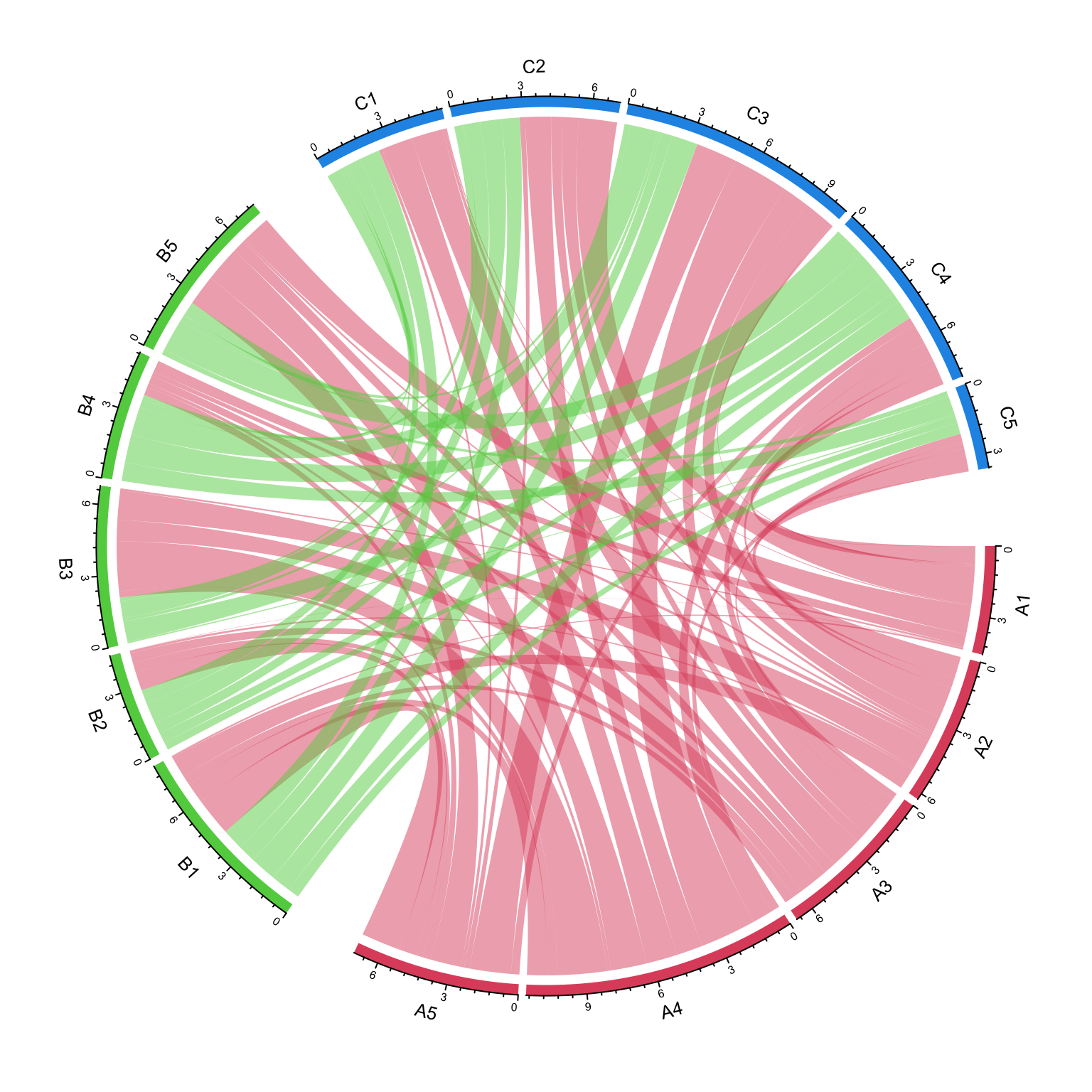
circos.clear()

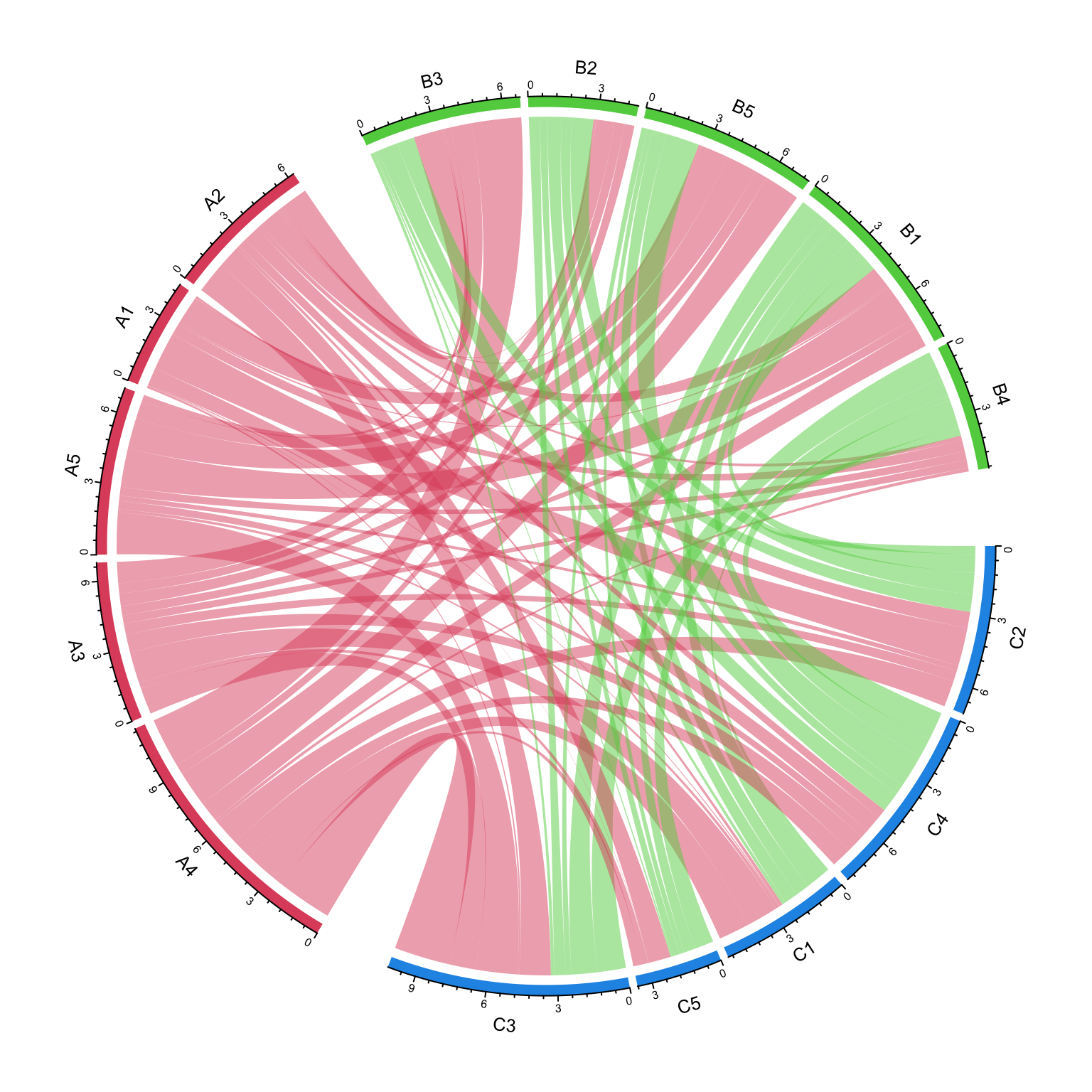
We can try another grouping:

group = structure(gsub("^\\w", "", nm), names = nm)
group

##  A1  A2  A3  A4  A5  B1  B2  B3  B4  B5  C1  C2  C3  C4  C5 
## "1" "2" "3" "4" "5" "1" "2" "3" "4" "5" "1" "2" "3" "4" "5"

chordDiagram(mat, group = group, grid.col = grid.col)

circos.clear()

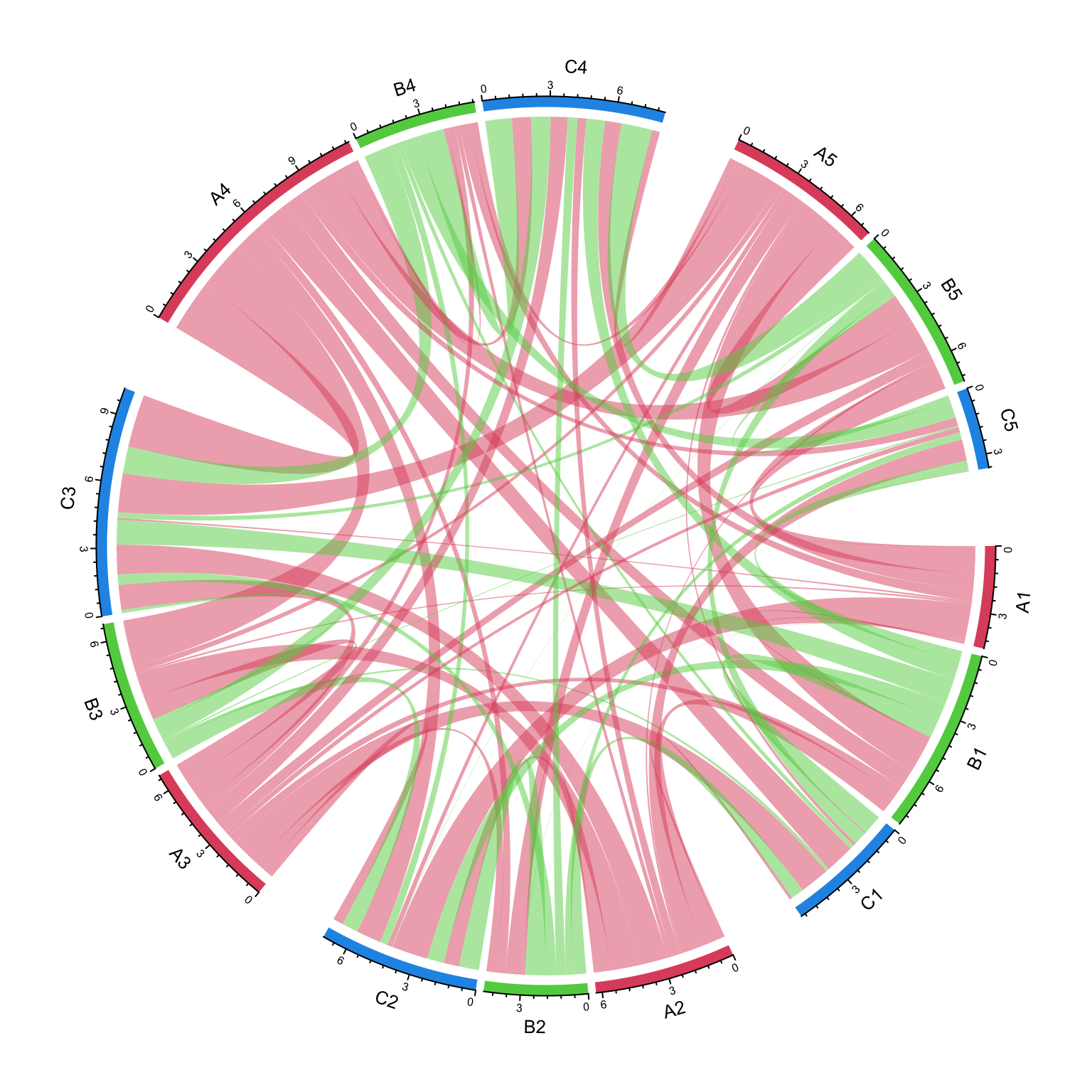
The order of group controls the sector orders and if group is set as a factor, the order of levels controls the order of groups.

group = structure(gsub("\\d", "", nm), names = nm)
group = factor(group[sample(length(group), length(group))], levels = c("C", "A", "B"))
group

## C4 C3 B2 C5 C2 B4 A4 B3 A3 A1 B1 C1 A2 B5 A5 
##  C  C  B  C  C  B  A  B  A  A  B  C  A  B  A 
## Levels: C A B

chordDiagram(mat, group = group, grid.col = grid.col)

circos.clear()

The gap between groups is controlled by big.gap argument and the gap between sectors is controlled by small.gap argument.

group = structure(gsub("\\d", "", nm), names = nm)
chordDiagram(mat, group = group, grid.col = grid.col, big.gap = 20, small.gap = 5)

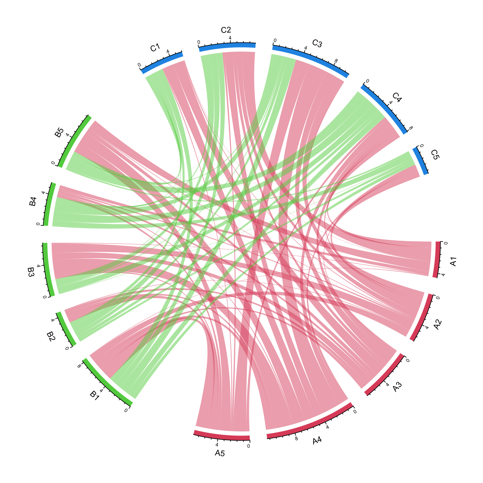
circos.clear()

As a normal Chord diagram, the labels and other tracks can be manually adjusted:

group = structure(gsub("\\d", "", nm), names = nm)
chordDiagram(mat, group = group, grid.col = grid.col,
	annotationTrack = c("grid", "axis"),
    preAllocateTracks = list(
        track.height = mm_h(4),
        track.margin = c(mm_h(4), 0)
))
circos.track(track.index = 2, panel.fun = function(x, y) {
    sector.index = get.cell.meta.data("sector.index")
    xlim = get.cell.meta.data("xlim")
    ylim = get.cell.meta.data("ylim")
    circos.text(mean(xlim), mean(ylim), sector.index, cex = 0.6, niceFacing = TRUE)
}, bg.border = NA)

highlight.sector(rownames(mat1), track.index = 1, col = "red", 
    text = "A", cex = 0.8, text.col = "white", niceFacing = TRUE)
highlight.sector(colnames(mat1), track.index = 1, col = "green", 
    text = "B", cex = 0.8, text.col = "white", niceFacing = TRUE)
highlight.sector(colnames(mat2), track.index = 1, col = "blue", 
    text = "C", cex = 0.8, text.col = "white", niceFacing = TRUE)

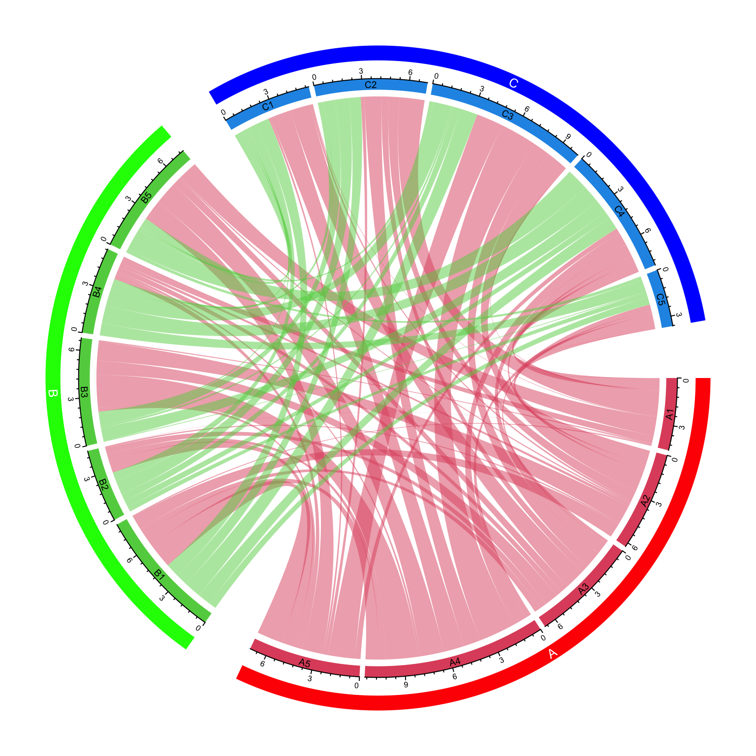
circos.clear()