Let’s first do a combination analysis with rGREAT and simplifyEnrichment. Let’s say, you have a list of genomic regions of interest (in the following example, we use a list of transcription factor binding sites). You do a GO enrichment analysis with rGREAT and visualize the enrichment results with simplifyEnrichment.
library(rGREAT)
df = read.table(url("https://raw.githubusercontent.com/jokergoo/rGREAT_suppl/master/data/tb_encTfChipPkENCFF708LCH_A549_JUN_hg19.bed"))
# convert to a GRanges object
gr = GRanges(seqnames = df[, 1], ranges = IRanges(df[, 2], df[, 3]))
res = great(gr, "BP", "hg19")
tb = getEnrichmentTable(res)
head(tb)
##           id                         description genome_fraction observed_region_hits
## 1 GO:0042981     regulation of apoptotic process       0.1420187                  386
## 2 GO:0043067 regulation of programmed cell death       0.1460764                  390
## 3 GO:0006915                   apoptotic process       0.1812937                  472
## 4 GO:0012501               programmed cell death       0.1860361                  481
## 5 GO:0033554         cellular response to stress       0.1564119                  404
## 6 GO:0008219                          cell death       0.1862993                  481
##   fold_enrichment p_value p_adjust mean_tss_dist observed_gene_hits gene_set_size
## 1        1.574712       0        0        125448                274          1427
## 2        1.546834       0        0        126430                279          1469
## 3        1.508407       0        0        124425                339          1883
## 4        1.497984       0        0        124981                349          1944
## 5        1.496479       0        0        134999                293          1812
## 6        1.495868       0        0        125470                350          1948
##   fold_enrichment_hyper p_value_hyper p_adjust_hyper
## 1              1.571393  2.220446e-15   5.315748e-13
## 2              1.554321  4.662937e-15   1.014825e-12
## 3              1.473356  9.769963e-15   1.913669e-12
## 4              1.469222  5.440093e-15   1.132485e-12
## 5              1.323329  1.098226e-07   3.529066e-06
## 6              1.470406  4.329870e-15   9.872103e-13
library(simplifyEnrichment)
sig_go_ids = tb$id[tb$p_adjust < 0.001]
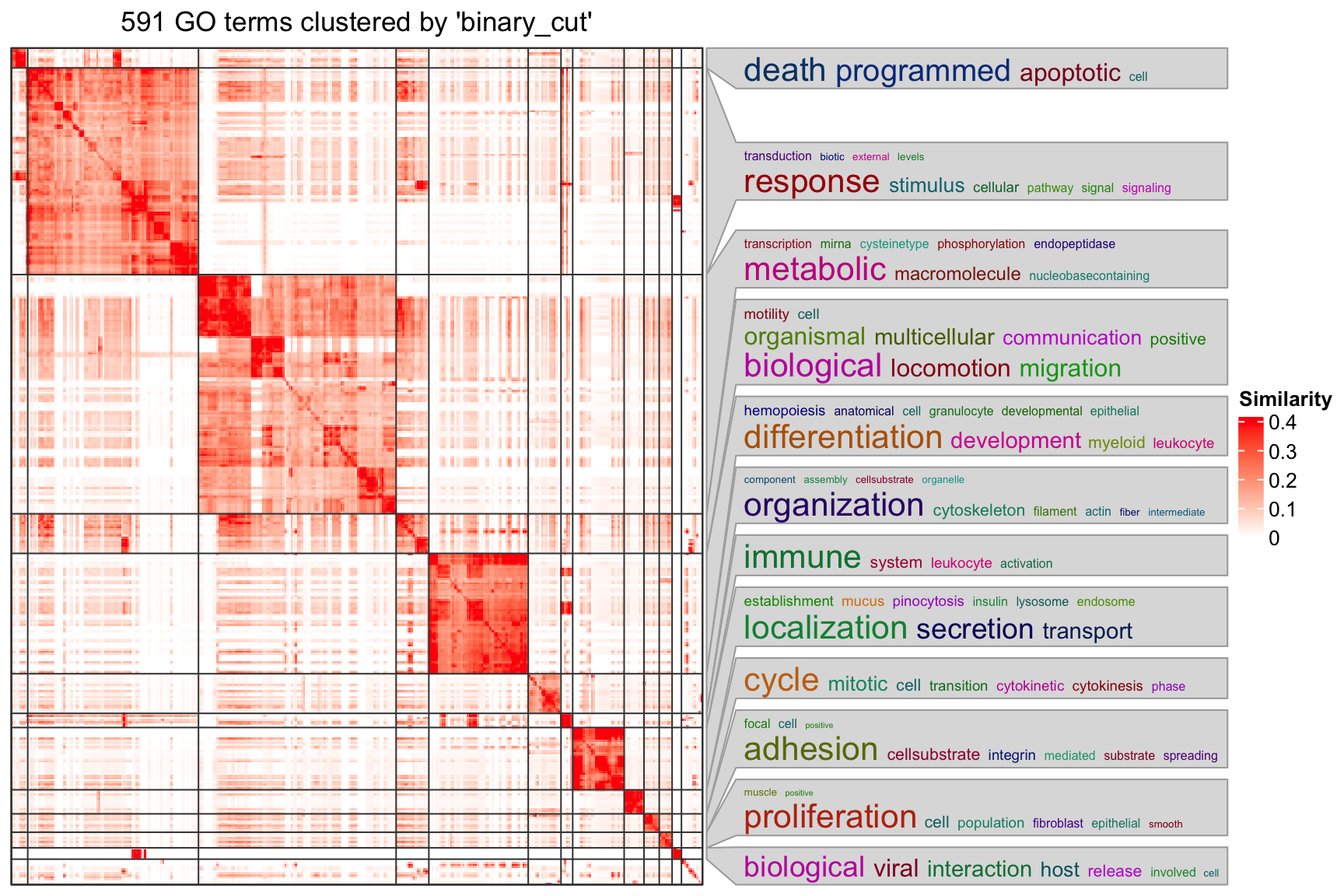
cl = simplifyGO(sig_go_ids)
head(cl)
##           id cluster
## 1 GO:0042981       1
## 2 GO:0043067       1
## 3 GO:0006915       1
## 4 GO:0012501       1
## 5 GO:0033554       2
## 6 GO:0008219       1
table(cl$cluster)
##
##   1   2   3   4   5   6   7   8   9  10  11  12  13  14  15  16  17  18  19  20  21  22
##  14 146 169   1   1  28  85  28  10  44  17  13   1   1  11   8   3   1   1   3   3   3
The plot looks not bad. Next you may want to get the gene-region associations for significant GO terms. For example, the association for the first GO term:
getRegionGeneAssociations(res, cl$id[1])
## GRanges object with 387 ranges and 2 metadata columns:
##         seqnames            ranges strand | annotated_genes    dist_to_TSS
##            <Rle>         <IRanges>  <Rle> | <CharacterList>  <IntegerList>
##     [1]     chr1 10003526-10003766      * |          NMNAT1             40
##     [2]     chr1 23073949-23074189      * |           KDM1A        -271752
##     [3]     chr1 23912118-23912358      * |             ID3         -25833
##     [4]     chr1 28479716-28479956      * |            EYA3         -64568
##     [5]     chr1 32420314-32420554      * |         KHDRBS1         -58741
##     ...      ...               ...    ... .             ...            ...
##   [383]    chr20 56273375-56273615      * |            ZBP1         -77743
##   [384]    chr20 62330537-62330777      * |        TNFRSF6B           3406
##   [385]    chr21 44897828-44898068      * |      SIK1,RRP1B -50826,-181364
##   [386]    chr22 37921455-37921695      * |          CARD10          -6077
##   [387]    chr22 50364455-50364695      * |            PIM3          10312
##   -------
##   seqinfo: 23 sequences from an unspecified genome; no seqlengths
There are more than 600 significant GO terms, and perhaps you don’t want to obtain such gene-region associations for every one of them.
As simplifyEnrichment already clusters significant GO terms into a smaller number of groups, you may switch your need of obtaining the associations from single GO terms to a group of GO terms where they show similar biological concept. In the new version of rGREAT (only available on GitHub currently), the second argument can be set as a vector of GO IDs. So, for example, to get the gene-region association for GO terms in the first cluster:
getRegionGeneAssociations(res, cl$id[cl$cluster == 1])
## GRanges object with 482 ranges and 2 metadata columns:
##         seqnames            ranges strand | annotated_genes    dist_to_TSS
##            <Rle>         <IRanges>  <Rle> | <CharacterList>  <IntegerList>
##     [1]     chr1   8254650-8254890      * |          ERRFI1        -168257
##     [2]     chr1 10003526-10003766      * |          NMNAT1             40
##     [3]     chr1 10440739-10440979      * |           KIF1B         169975
##     [4]     chr1 16472855-16473095      * |           EPHA2           9487
##     [5]     chr1 16490874-16491114      * |           EPHA2          -8292
##     ...      ...               ...    ... .             ...            ...
##   [478]    chr20 62330537-62330777      * |        TNFRSF6B           3406
##   [479]    chr21 44897828-44898068      * |      SIK1,RRP1B -50826,-181364
##   [480]    chr22 21258958-21259198      * |            CRKL         -12516
##   [481]    chr22 37921455-37921695      * |          CARD10          -6077
##   [482]    chr22 50364455-50364695      * |            PIM3          10312
##   -------
##   seqinfo: 23 sequences from an unspecified genome; no seqlengths
SessionInfo
sessionInfo()
## R version 4.4.2 (2024-10-31)
## Platform: aarch64-apple-darwin20
## Running under: macOS 26.0.1
##
## Matrix products: default
## BLAS:   /Library/Frameworks/R.framework/Versions/4.4-arm64/Resources/lib/libRblas.0.dylib
## LAPACK: /Library/Frameworks/R.framework/Versions/4.4-arm64/Resources/lib/libRlapack.dylib;  LAPACK version 3.12.0
##
## locale:
## [1] C.UTF-8/UTF-8/C.UTF-8/C/C.UTF-8/C.UTF-8
##
## time zone: Europe/Berlin
## tzcode source: internal
##
## attached base packages:
## [1] stats4    stats     graphics  grDevices utils     datasets  methods   base
##
## other attached packages:
## [1] simplifyEnrichment_2.0.0 rGREAT_2.8.0             GenomicRanges_1.58.0
## [4] GenomeInfoDb_1.42.3      IRanges_2.40.1           S4Vectors_0.44.0
## [7] BiocGenerics_0.52.0      knitr_1.50               colorout_1.3-2
##
## loaded via a namespace (and not attached):
##   [1] DBI_1.2.3                                bitops_1.0-9
##   [3] rlang_1.1.5                              magrittr_2.0.3
##   [5] clue_0.3-66                              GetoptLong_1.0.5
##   [7] flexclust_1.5.0                          matrixStats_1.5.0
##   [9] compiler_4.4.2                           RSQLite_2.3.9
##  [11] GenomicFeatures_1.58.0                   png_0.1-8
##  [13] vctrs_0.6.5                              pkgconfig_2.0.3
##  [15] shape_1.4.6.1                            crayon_1.5.3
##  [17] fastmap_1.2.0                            magick_2.8.5
##  [19] XVector_0.46.0                           Rsamtools_2.22.0
##  [21] promises_1.3.2                           rmarkdown_2.29
##  [23] UCSC.utils_1.2.0                         bit_4.5.0.1
##  [25] modeltools_0.2-24                        xfun_0.51
##  [27] zlibbioc_1.52.0                          cachem_1.1.0
##  [29] jsonlite_1.9.0                           progress_1.2.3
##  [31] blob_1.2.4                               later_1.4.1
##  [33] DelayedArray_0.32.0                      BiocParallel_1.40.0
##  [35] parallel_4.4.2                           prettyunits_1.2.0
##  [37] cluster_2.1.6                            R6_2.6.1
##  [39] bslib_0.9.0                              RColorBrewer_1.1-3
##  [41] rtracklayer_1.66.0                       jquerylib_0.1.4
##  [43] Rcpp_1.0.14                              bookdown_0.44
##  [45] SummarizedExperiment_1.36.0              iterators_1.0.14
##  [47] httpuv_1.6.15                            Matrix_1.7-1
##  [49] igraph_2.1.4                             abind_1.4-8
##  [51] yaml_2.3.10                              doParallel_1.0.17
##  [53] codetools_0.2-20                         blogdown_1.19
##  [55] curl_6.2.1                               lattice_0.22-6
##  [57] Biobase_2.66.0                           shiny_1.10.0
##  [59] KEGGREST_1.46.0                          evaluate_1.0.3
##  [61] xml2_1.3.6                               circlize_0.4.16
##  [63] Biostrings_2.74.1                        MatrixGenerics_1.18.1
##  [65] TxDb.Hsapiens.UCSC.hg19.knownGene_3.2.2  DT_0.33
##  [67] foreach_1.5.2                            NLP_0.3-2
##  [69] RCurl_1.98-1.16                          hms_1.1.3
##  [71] xtable_1.8-4                             class_7.3-22
##  [73] slam_0.1-55                              scatterplot3d_0.3-44
##  [75] tools_4.4.2                              BiocIO_1.16.0
##  [77] tm_0.7-16                                TxDb.Hsapiens.UCSC.hg38.knownGene_3.20.0
##  [79] GenomicAlignments_1.42.0                 XML_3.99-0.18
##  [81] Cairo_1.6-2                              fastmatch_1.1-6
##  [83] grid_4.4.2                               AnnotationDbi_1.68.0
##  [85] colorspace_2.1-1                         GenomeInfoDbData_1.2.13
##  [87] restfulr_0.0.15                          cli_3.6.4
##  [89] Polychrome_1.5.1                         S4Arrays_1.6.0
##  [91] ComplexHeatmap_2.25.2                    sass_0.4.9
##  [93] digest_0.6.37                            SparseArray_1.6.2
##  [95] org.Hs.eg.db_3.20.0                      rjson_0.2.23
##  [97] htmlwidgets_1.6.4                        memoise_2.0.1
##  [99] htmltools_0.5.8.1                        simona_1.7.1
## [101] lifecycle_1.0.4                          httr_1.4.7
## [103] GlobalOptions_0.1.2                      GO.db_3.20.0
## [105] mime_0.12                                bit64_4.6.0-1