Integrate ComplexHeatmap with cowplot package

The cowplot package is used to combine multiple plots into a single figure. In most cases, ComplexHeatmap works perfectly with cowplot, but there are some cases that need special attention.

Also there are some other packages that combine multiple plots, such as multipanelfigure, but I think the mechanism behind is the same.

Following functionalities in ComplexHeatmap cause problems with using cowplot.

anno_zoom()/anno_link(). The adjusted positions by these two functions rely on the size of the graphics device.
anno_mark(). The same reason as anno_zoom(). The adjusted positions also rely on the device size.
When there are too many legends, the legends will be wrapped into multiple columns. The calculation of the legend positions rely on the device size.

In following I demonstrate a case with using the anno_zoom(). Here the example is from the simplifyEnrichment package and the plot shows a GO similarity heatmap with word cloud annotation showing the major biological functions in each group.

You don’t need to really understand the following code. The ht_clusters() function basically draws a heatmap with Heatmap() and add the word cloud annotation by anno_zoom().

library(simplifyEnrichment)
set.seed(1234)
go_id = random_GO(500)
mat = GO_similarity(go_id)
cl = binary_cut(mat)
ht_clusters(mat, cl)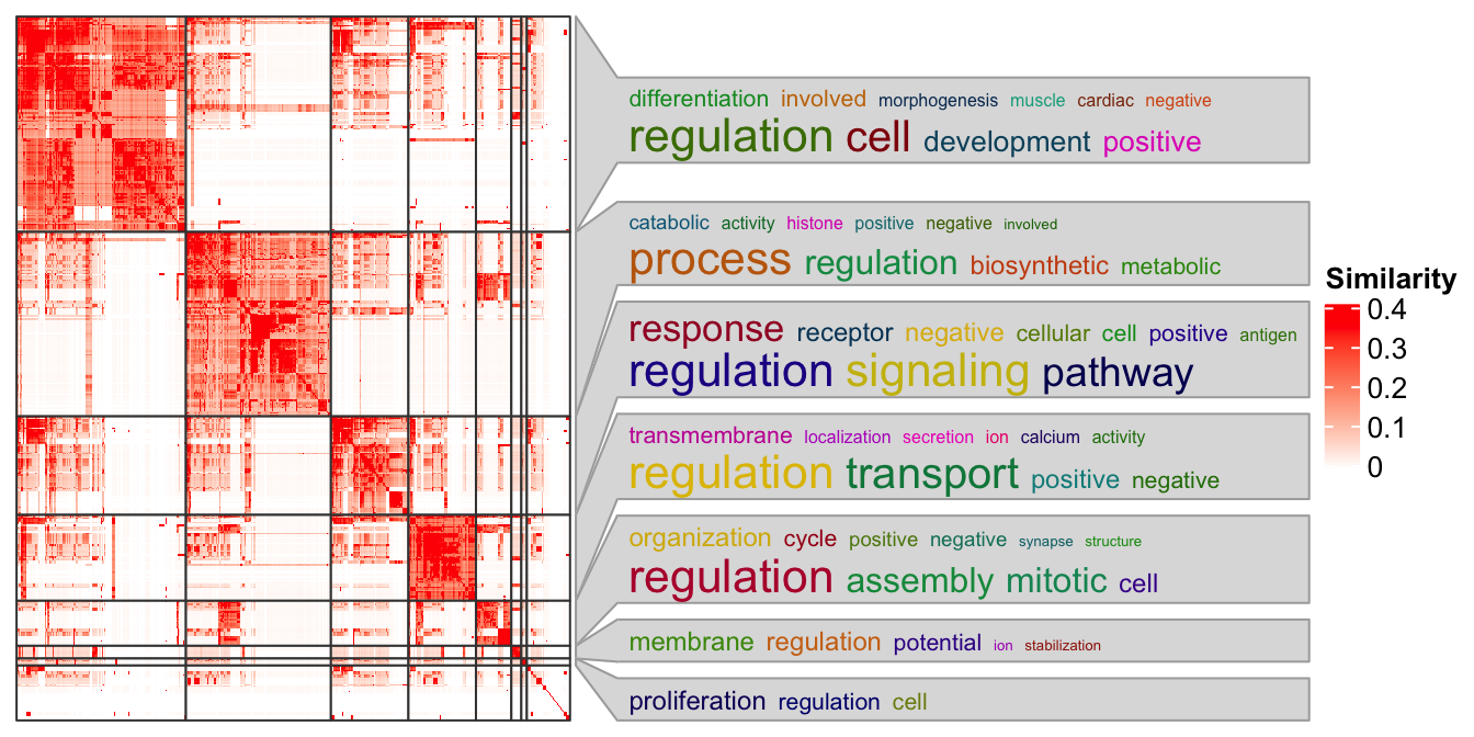

Next we put this heatmap as a sub-figure with cowplot. To integrate with cowplot, the heatmap should be captured by grid::grid.grabExpr() as a complex grob object. Note here you need to use draw() function to draw the heatmap explicitly.

library(cowplot)
library(grid)
p1 = rectGrob(width = 0.9, height = 0.9)
p2 = grid.grabExpr(ht_clusters(mat, cl))
p3 = rectGrob(width = 0.9, height = 0.9)

plot_grid(p1, 
    plot_grid(p2, p3, nrow = 2, rel_heights = c(4, 1)), 
    nrow = 1, rel_widths = c(1, 9)
)

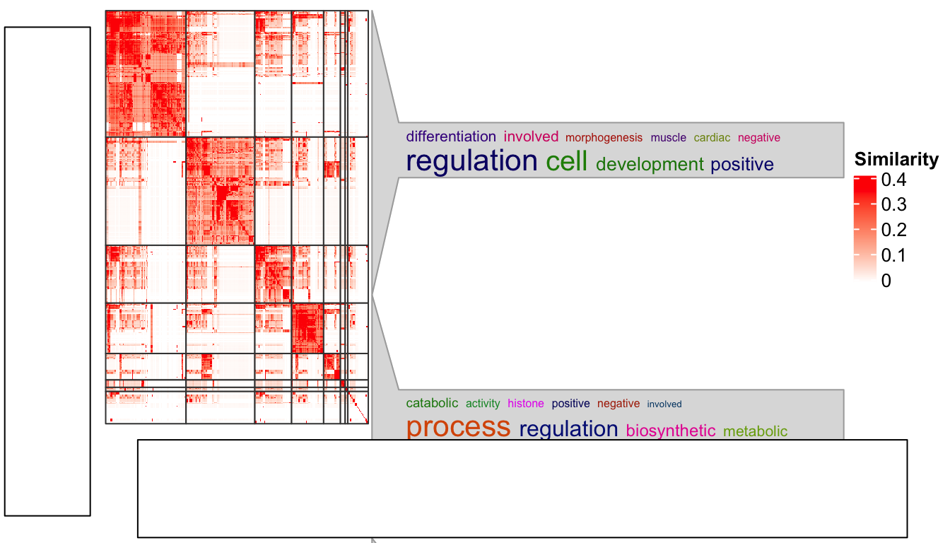
Woooo! The word cloud annotation is badly aligned.

There are some details that should be noted for grid.grabExpr() function. It actually opens an invisible graphics device (by pdf(NULL)) with a default size 7x7 inches. Thus, for this line:

p2 = grid.grabExpr(ht_clusters(mat, cl))

The word cloud annotation in p2 is actually calculated in a region of 7x7 inches, and when it is written back to the figure by plot_grid(), the space for p2 changes, that is why the word cloud annotation is wrongly aligned.

On the other hand, if “a simple heatmap” is captured by grid.grabExpr(), e.g.:

p2 = grid.grabExpr(draw(Heatmap(mat)))

when p2 is put back, everything will work fine because now all the heatmap elements are not dependent on the device size and the positions will be automatically adjusted to the new space.

This effect can also be observed by plotting the heatmap in the interactive graphics device and resizing the window by dragging it.

The solution is rather simple. Since the reason for this inconsistency is the different space between where it is captured and where it is drawn, we only need to capture the heatmap under the device with the same size as where it is going to be put.

As in the layout which we set in the plot_grid() function, the heatmap occupies 9/10 width and 4/5 height of the figure. So, the width and height of the space for the heatmap is calculated as follows and assigned to the width and height arguments in grid.grabExpr().

w = convertWidth(unit(1, "npc")*(9/10), "inch", valueOnly = TRUE)
h = convertHeight(unit(1, "npc")*(4/5), "inch", valueOnly = TRUE)
p2 = grid.grabExpr(ht_clusters(mat, cl), width = w, height = h)

plot_grid(p1, 
    plot_grid(p2, p3, nrow = 2, rel_heights = c(4, 1)), 
    nrow = 1, rel_widths = c(1, 9)
)

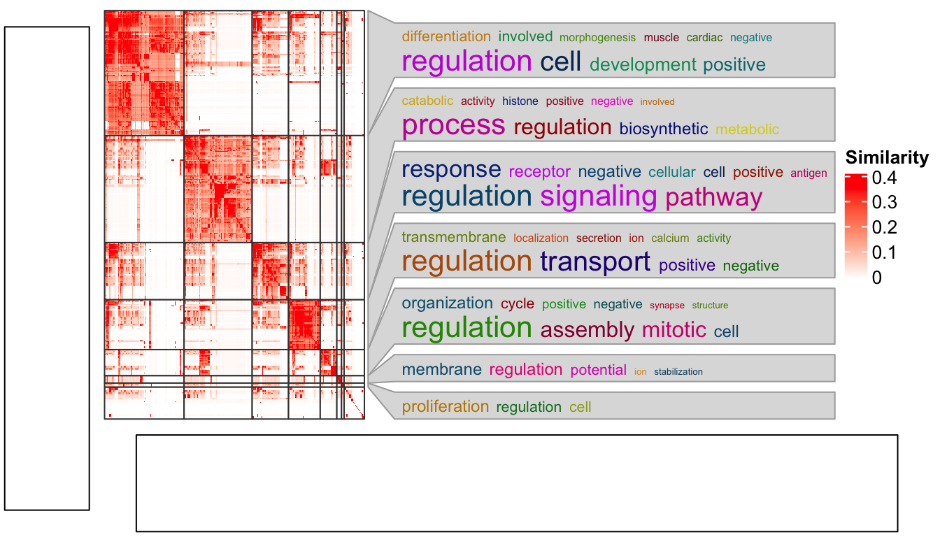
Now everthing is back to normal!