3 Heatmap Annotations

Heatmap annotations are important components of a heatmap that it shows additional information that associates with rows or columns in the heatmap. ComplexHeatmap package provides very flexible supports for setting annotations and defining new annotation graphics. The annotations can be put on the four sides of the heatmap, by top_annotation, bottom_annotation, left_annotation and right_annotation arguments.

The value for the four arguments should be in the HeatmapAnnotation class and should be constructed by HeatmapAnnotation() function, or by rowAnnotation() function if it is a row annotation. (rowAnnotation() is just a helper function which is identical to HeatmapAnnotation(..., which = "row")). A simple usage of heatmap annotations is as follows.

set.seed(123)
mat = matrix(rnorm(100), 10)
rownames(mat) = paste0("R", 1:10)
colnames(mat) = paste0("C", 1:10)
column_ha = HeatmapAnnotation(foo1 = runif(10), bar1 = anno_barplot(runif(10)))
row_ha = rowAnnotation(foo2 = runif(10), bar2 = anno_barplot(runif(10)))
Heatmap(mat, name = "mat", top_annotation = column_ha, right_annotation = row_ha)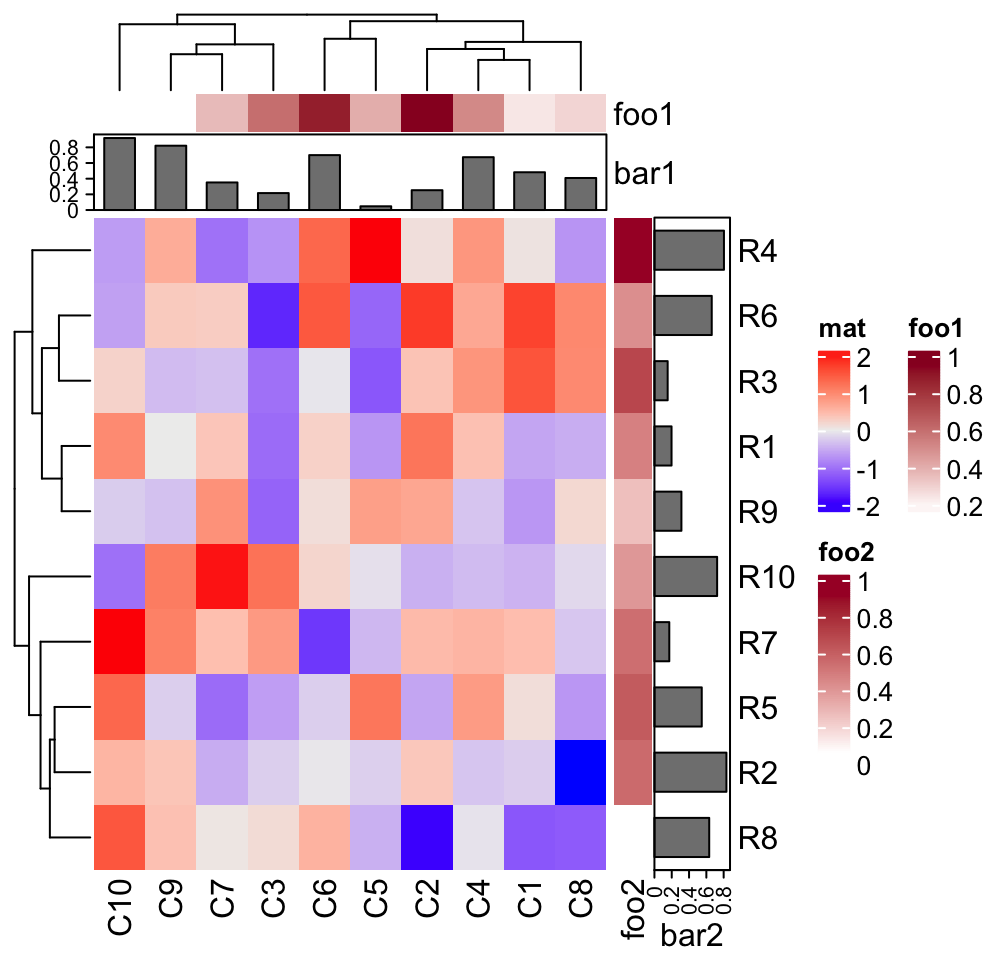

Or assign as bottom annotation and left annotation.

Heatmap(mat, name = "mat", bottom_annotation = column_ha, left_annotation = row_ha)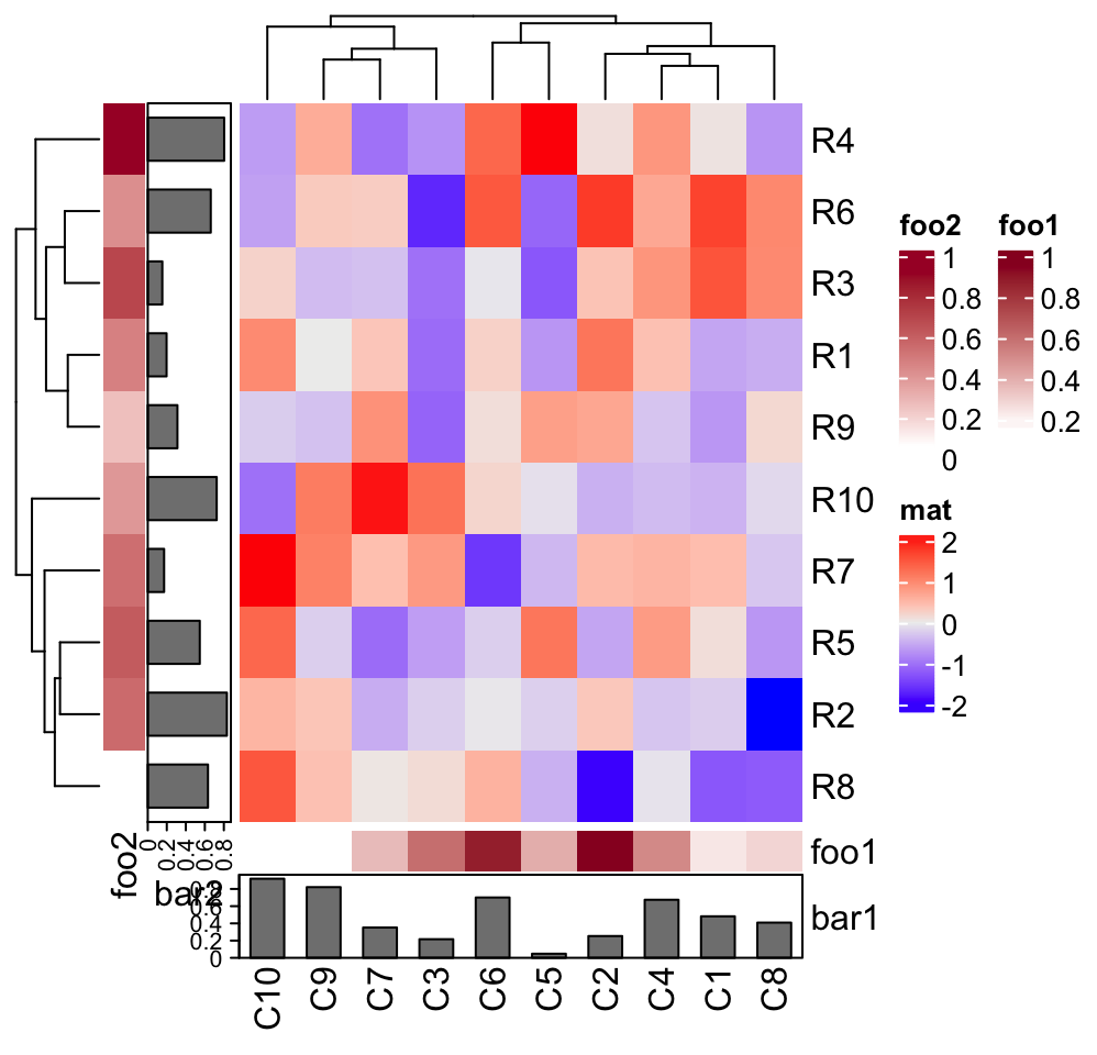

In above examples, column_ha and row_ha both have two annotations where foo1 and foo2 are numeric vectors and bar1 and bar2 are barplots. The vector-like annotation is called “simple annotation” here and the barplot annotation is called “complex annotation”. You can already see the annotations must be defined as name-value pairs (e.g. foo = ...).

Heatmap annotations can also be independent of the heatmaps. They can be concatenated to the heatmap list by + if it is horizontal, or %v% if it is vertical. Chapter 4 will discuss how to concatenate heatmaps and annotations.

# code only for demonstration
Heatmap(...) + rowAnnotation() + ...
Heatmap(...) %v% HeatmapAnnotation(...) %v% ...

HeatmapAnnotation() returns a HeatmapAnnotation class object. The object is usually composed of several annotations. In the following sections of this chapter, we first introduce settings for individal annotation, and later we show how to put them toghether.

You can see the information of the column_ha and row_ha objects by directly enter the object names:

column_ha

## A HeatmapAnnotation object with 2 annotations
##   name: heatmap_annotation_0 
##   position: column 
##   items: 10 
##   width: 1npc 
##   height: 15.3514598035146mm 
##   this object is subsettable
##   5.92288888888889mm extension on the left 
##   9.4709mm extension on the right 
## 
##  name   annotation_type color_mapping height
##  foo1 continuous vector        random    5mm
##  bar1    anno_barplot()                 10mm

row_ha

## A HeatmapAnnotation object with 2 annotations
##   name: heatmap_annotation_1 
##   position: row 
##   items: 10 
##   width: 15.3514598035146mm 
##   height: 1npc 
##   this object is subsettable
##   9.96242222222222mm extension on the bottom 
## 
##  name   annotation_type color_mapping width
##  foo2 continuous vector        random   5mm
##  bar2    anno_barplot()                10mm

In the following examples in this chapter, we will only show the graphics for the annotations with no heatmap, unless it is necessary. If you want to try it with a heatmap, you just assign the HeatmapAnnotation object which we always name as ha to top_annotation, bottom_annotation, left_annotation or right_annotation arguments.

Settings are basically the same for column annotations and row annotations. If there is nothing specicial, we only show the column annotation as examples. If you want to try row annotation, just add which = "row" to HeatmapAnnotation() or directly change to rowAnnotation() function.

3.1 Simple annotation

A so-called “simple annotation” is the most used style of annotations which is heatmap-like or grid-like graphics where colors are used to map to the annotation values. To generate a simple annotation, you just simply put the annotation vector in HeatmapAnnotation() with a certain name.

ha = HeatmapAnnotation(foo = 1:10)

Or a discrete annotation:

ha = HeatmapAnnotation(bar = sample(letters[1:3], 10, replace = TRUE))

You can use any strings as annotation names except those pre-defined arguments in HeatmapAnnotation().

If colors are not specified, colors are randomly generated. To set colors for annotations, col needs to be set as a named list where the names should be the same as annotation names. For continuous values, the color mapping should be a color mapping function generated by circlize::colorRamp2().

library(circlize)
col_fun = colorRamp2(c(0, 5, 10), c("blue", "white", "red"))
ha = HeatmapAnnotation(foo = 1:10, col = list(foo = col_fun))

And for discrete annotations, the color should be a named vector where names correspond to the levels in the annotation.

ha = HeatmapAnnotation(bar = sample(letters[1:3], 10, replace = TRUE),
    col = list(bar = c("a" = "red", "b" = "green", "c" = "blue")))

If you specify more than one vectors, there will be multiple annotations (foo and bar in following example). Also you can see how col is set when foo and bar are all put into a single HeatmapAnnotation(). Maybe now you can understand the names in the color list is actually used to map to the annotation names. Values in col will be used to construct legends for simple annotations.

ha = HeatmapAnnotation(
    foo = 1:10, 
    bar = sample(letters[1:3], 10, replace = TRUE),
    col = list(foo = col_fun,
               bar = c("a" = "red", "b" = "green", "c" = "blue")
    )
)

The color for NA value is controlled by na_col argument.

ha = HeatmapAnnotation(
    foo = c(1:4, NA, 6:10), 
    bar = c(NA, sample(letters[1:3], 9, replace = TRUE)),
    col = list(foo = col_fun,
               bar = c("a" = "red", "b" = "green", "c" = "blue")
    ),
    na_col = "black"
)

gp mainly controls the graphics parameters for the borders of the grids.

ha = HeatmapAnnotation(
    foo = 1:10, 
    bar = sample(letters[1:3], 10, replace = TRUE),
    col = list(foo = col_fun,
               bar = c("a" = "red", "b" = "green", "c" = "blue")
    ),
    gp = gpar(col = "black")
)

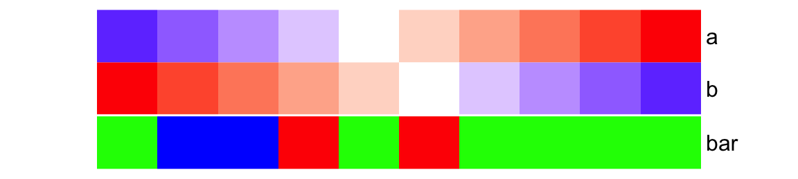
The simple annotation can also be a matrix (numeric or character) that all the columns in the matrix share a same color mapping schema. Note columns in the matrix correspond to the rows in the column annotation (you can imagine a vector is a one-column matrix). Also the column names of the matrix are used as the annotation names.

ha = HeatmapAnnotation(foo = cbind(a = runif(10), b = runif(10)))

If the matrix has no column name, the name of the annotation is still used, but drawn in the middle of the annotation.

ha = HeatmapAnnotation(foo = cbind(runif(10), runif(10)))

As simple annotations can be in different modes (e.g. numeric, or character), they can be combined as a data frame and send to df argument. Imagine in your project, you might already have an annotation table, you can directly set it by df.

anno_df = data.frame(
    foo = 1:10,
    bar = sample(letters[1:3], 10, replace = TRUE)
)
ha = HeatmapAnnotation(df = anno_df,
    col = list(foo = col_fun,
               bar = c("a" = "red", "b" = "green", "c" = "blue")
    )
)

Single annotations and data frame can be mixed, but single annotations are inserted after the data frame annotation. In following example, colors for foo2 is not specified, random colors will be used.

ha = HeatmapAnnotation(df = anno_df,
    foo2 = rnorm(10),
    col = list(foo = col_fun,
               bar = c("a" = "red", "b" = "green", "c" = "blue")
    )
)

border controls the border of every single annotation.

ha = HeatmapAnnotation(
    foo = cbind(1:10, 10:1),
    bar = sample(letters[1:3], 10, replace = TRUE),
    col = list(foo = col_fun,
               bar = c("a" = "red", "b" = "green", "c" = "blue")
    ),
    border = TRUE
)

The height of the simple annotation is controlled by simple_anno_size argument. Since all single annotations have same height, the value of simple_anno_size is a single unit value. Note there are arguments like width, height, annotation_width and annotation_height, but they are used to adjust the width/height for the complete heamtap annotations (which are always mix of several annotations). The adjustment of these four arguments will be introduced in Section 3.21.

ha = HeatmapAnnotation(
    foo = cbind(a = 1:10, b = 10:1), 
    bar = sample(letters[1:3], 10, replace = TRUE),
    col = list(foo = col_fun,
               bar = c("a" = "red", "b" = "green", "c" = "blue")
    ),
    simple_anno_size = unit(1, "cm")
)

When you have multiple heatmaps and it is better to keep the size of simple annotations on all heatmaps with the same size. ht_opt$simple_anno_size can be set to control the simple annotation size globally (It will be introduced in Section 4.13).

3.2 Simple annotation as an annotation function

HeatmapAnnotation() supports “complex annotation” by setting the annotation as a function. The annotation function defines how to draw the graphics at a certain position corresponding to the column or row in the heatmap. There are quite a lot of annotation functions predefined in ComplexHeatmap package. In the end of this chapter, we will introduce how to construct your own annotation function by the AnnotationFunction class.

For all the annotation functions in forms of anno_*(), if it is specified in HeatmapAnnotation() or rowAnnotation(), you don’t need to do anything explicitly on anno_*() to tell whether it should be drawn on rows or columns. anno_*() automatically detects whether it is a row annotation environment or a column annotation environment.

The simple annotation shown in previous section is internally constructed by anno_simple() annotation function. Directly using anno_simple() will not automatically generate legends for the final plot, but, it can provide more flexibility for more annotation graphics (note in Chapter 5 we will show, although anno_simple() cannot automatically generate the legends, the legends can be controlled and added to the final plot manually).

For an example in previous section:

# code only for demonstration
ha = HeatmapAnnotation(foo = 1:10)

is actually identical to:

# code only for demonstration
ha = HeatmapAnnotation(foo = anno_simple(1:10))

anno_simple() makes heatmap-like annotations (or the simple annotations). Basically if users only make heatmap-like annotations, they do not need to directly use anno_simple(), but this function allows to add more symbols on the annotation grids.

anno_simple() allows to add “points” or single-letter symbols on top of the annotation grids. pch, pt_gp and pt_size control the settings of the points. The value of pch can be a vector with possible NA values.

ha = HeatmapAnnotation(foo = anno_simple(1:10, pch = 1, 
    pt_gp = gpar(col = "red"), pt_size = unit(1:10, "mm")))

Set pch as a vector:

ha = HeatmapAnnotation(foo = anno_simple(1:10, pch = 1:10))

Set pch as a vector of letters:

ha = HeatmapAnnotation(foo = anno_simple(1:10, 
    pch = sample(letters[1:3], 10, replace = TRUE)))

Set pch as a vector with NA values (nothing is drawn for NA pch values):

ha = HeatmapAnnotation(foo = anno_simple(1:10, pch = c(1:4, NA, 6:8, NA, 10, 11)))

pch also works if the value for anno_simple() is a matrix. The length of pch should be as same as the number of matrix rows or columns or even the length of the matrix (the length of the matrix is the length of all data points in the matrix).

Length of pch corresponds to matrix columns:

ha = HeatmapAnnotation(foo = anno_simple(cbind(1:10, 10:1), pch = 1:2))

Length of pch corresponds to matrix rows:

ha = HeatmapAnnotation(foo = anno_simple(cbind(1:10, 10:1), pch = 1:10))

pch is a matrix:

pch = matrix(1:20, nc = 2)
pch[sample(length(pch), 10)] = NA
ha = HeatmapAnnotation(foo = anno_simple(cbind(1:10, 10:1), pch = pch))

Till now, you might wonder how to set the legends of the symbols you’ve added to the simple annotations. Here we will only show you a simple example and this functionality will be discussed in Chapter 5. In following example, we assume the simple annotations are kind of p-values and we add * for p-values less than 0.01.

set.seed(123)
pvalue = 10^-runif(10, min = 0, max = 3)
is_sig = pvalue < 0.01
pch = rep("*", 10)
pch[!is_sig] = NA
# color mapping for -log10(pvalue)
pvalue_col_fun = colorRamp2(c(0, 2, 3), c("green", "white", "red")) 
ha = HeatmapAnnotation(
    pvalue = anno_simple(-log10(pvalue), col = pvalue_col_fun, pch = pch),
    annotation_name_side = "left")
ht = Heatmap(matrix(rnorm(100), 10), name = "mat", top_annotation = ha)
# now we generate two legends, one for the p-value
# see how we define the legend for pvalue
lgd_pvalue = Legend(title = "p-value", col_fun = pvalue_col_fun, at = c(0, 1, 2, 3), 
    labels = c("1", "0.1", "0.01", "0.001"))
# and one for the significant p-values
lgd_sig = Legend(pch = "*", type = "points", labels = "< 0.01")
# these two self-defined legends are added to the plot by `annotation_legend_list`
draw(ht, annotation_legend_list = list(lgd_pvalue, lgd_sig))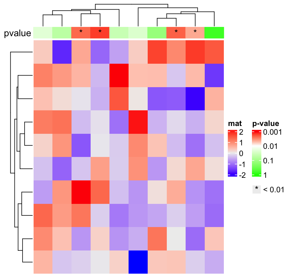

The height of the simple annotation can be controlled by height argument or simple_anno_size inside anno_simple(). simple_anno_size controls the size for single-row annotation and height/width controls the total height/width of the simple annotations. If height/width is set, simple_anno_size is ignored.

ha = HeatmapAnnotation(foo = anno_simple(1:10, height = unit(2, "cm")))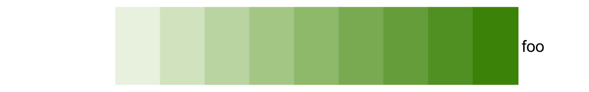

ha = HeatmapAnnotation(foo = anno_simple(cbind(1:10, 10:1), 
    simple_anno_size = unit(2, "cm")))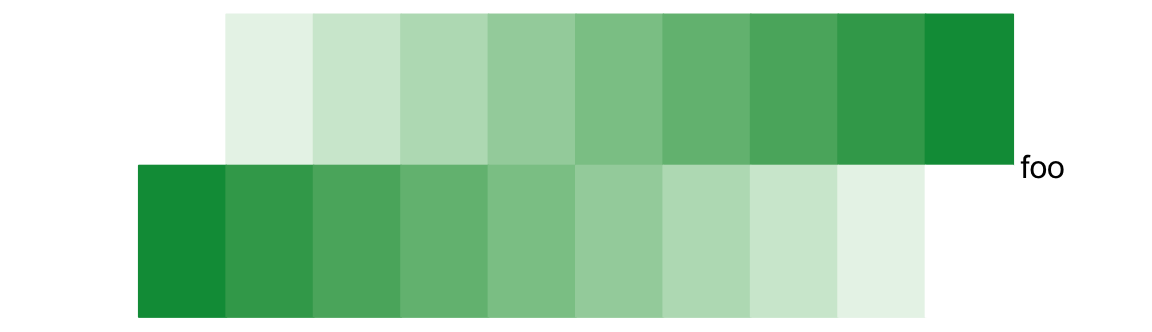

For all the annotation functions we introduce later, the height or the width for individual annotations should all be set inside the anno_*() functions.

# code only for demonstration
anno_*(..., width = ...)
anno_*(..., height = ...)

Again, the width, height, annotation_width and annotation_height arguments in HeatmapAnnotation() are used to adjust the size of multiple annotations.

3.3 Empty annotation

anno_empty() is a place holder where nothing is drawn. Later user-defined graphics can be added by decorate_annotation() function.

ha = HeatmapAnnotation(foo = anno_empty(border = TRUE))

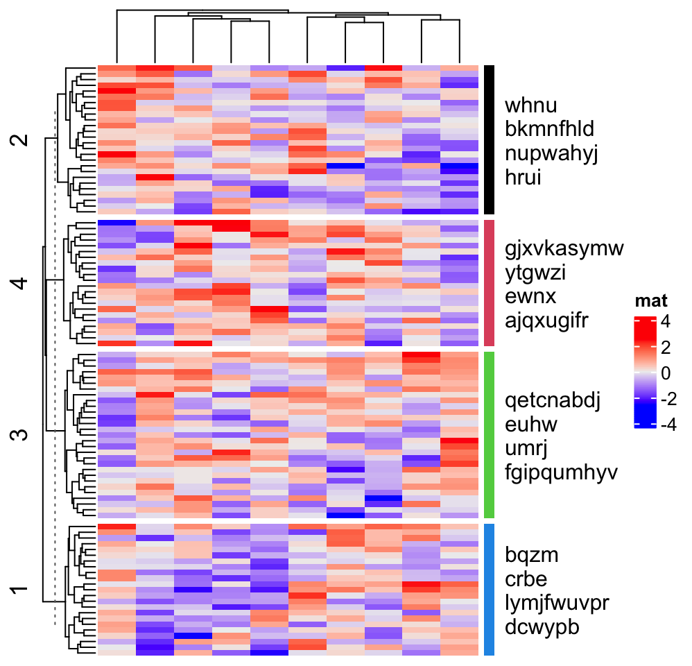
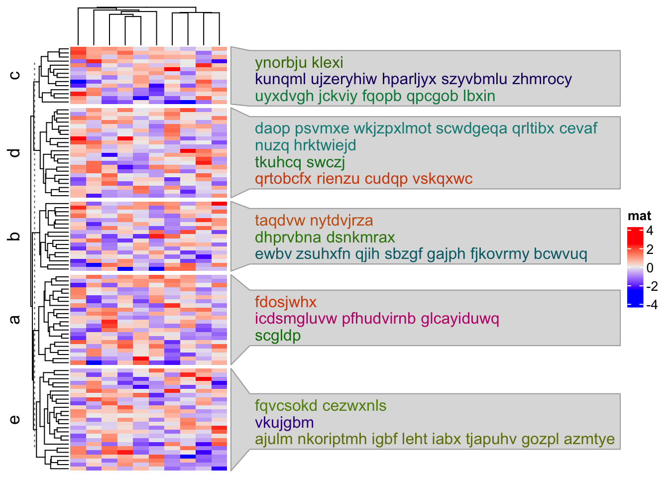
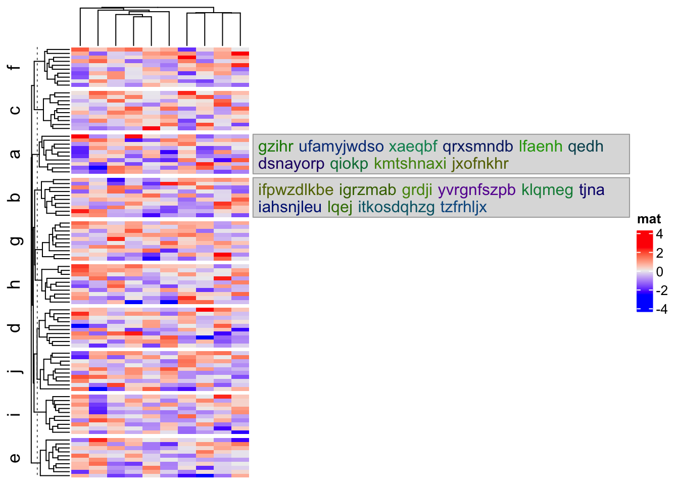
In Chapter 6, we will introduce the use of the decoration functions, but here we give a quick example. In gene expression expression analysis, there are senarios that we split the heatmaps into several groups and we want to highlight some key genes in each group. In this case, we simply add the gene names on the right side of the heatmap without aligning them to the their corresponding rows. (anno_mark() can align the labels correclty to their corresponding rows, but in the example we show here, it is not necessray).

In following example, since rows are split into four slices, the empty annotation is also split into four slices. Basically what we do is in each empty annotation slice, we add a colored segment and text.

random_text = function(n) {
    sapply(1:n, function(i) {
        paste0(sample(letters, sample(4:10, 1)), collapse = "")
    })
}
text_list = list(
    text1 = random_text(4),
    text2 = random_text(4),
    text3 = random_text(4),
    text4 = random_text(4)
)
# note how we set the width of this empty annotation
ha = rowAnnotation(foo = anno_empty(border = FALSE, 
    width = max_text_width(unlist(text_list)) + unit(4, "mm")))
Heatmap(matrix(rnorm(1000), nrow = 100), name = "mat", row_km = 4, right_annotation = ha)
for(i in 1:4) {
    decorate_annotation("foo", slice = i, {
        grid.rect(x = 0, width = unit(2, "mm"), gp = gpar(fill = i, col = NA), just = "left")
        grid.text(paste(text_list[[i]], collapse = "\n"), x = unit(4, "mm"), just = "left")
    })
}

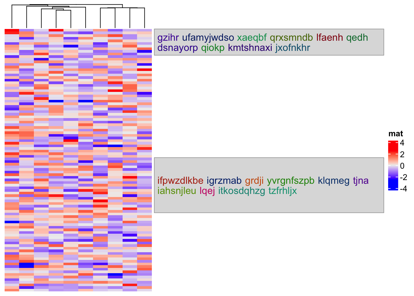
Note the previous plot can also be made by anno_block() or anno_textbox() (Section 3.19).

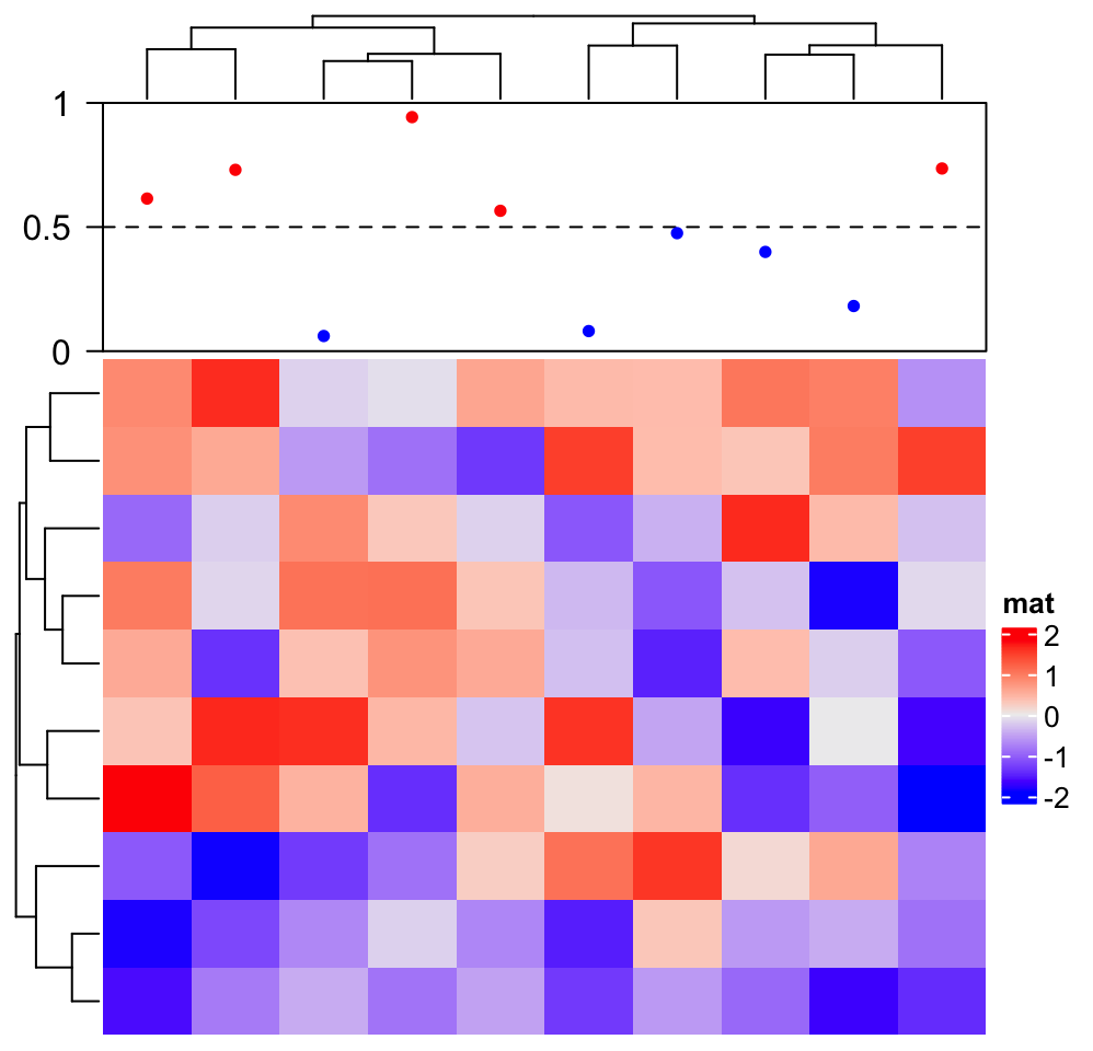
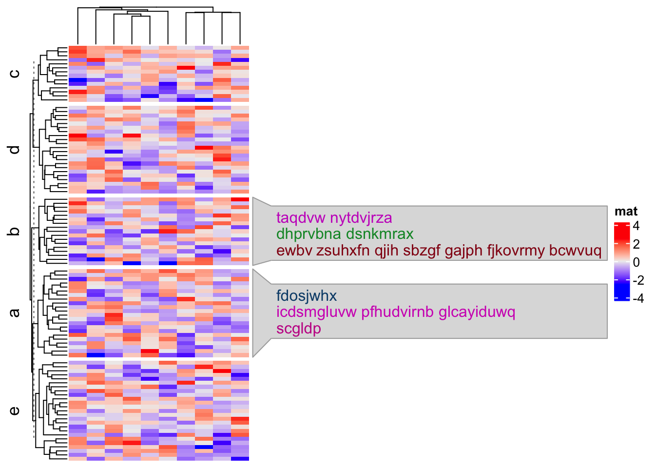
A second use of the empty annotation is to add complex annotation graphics where the empty annotation pretends to be a virtual plotting region. You can construct an annotation function by AnnotationFunction class for complex annotation graphics, which allows subsetting and splitting, but still, it can be a secondary choice to directly draw inside the empty annotation, which is easier and faster for implementing (but less flexible and does not allow splitting).

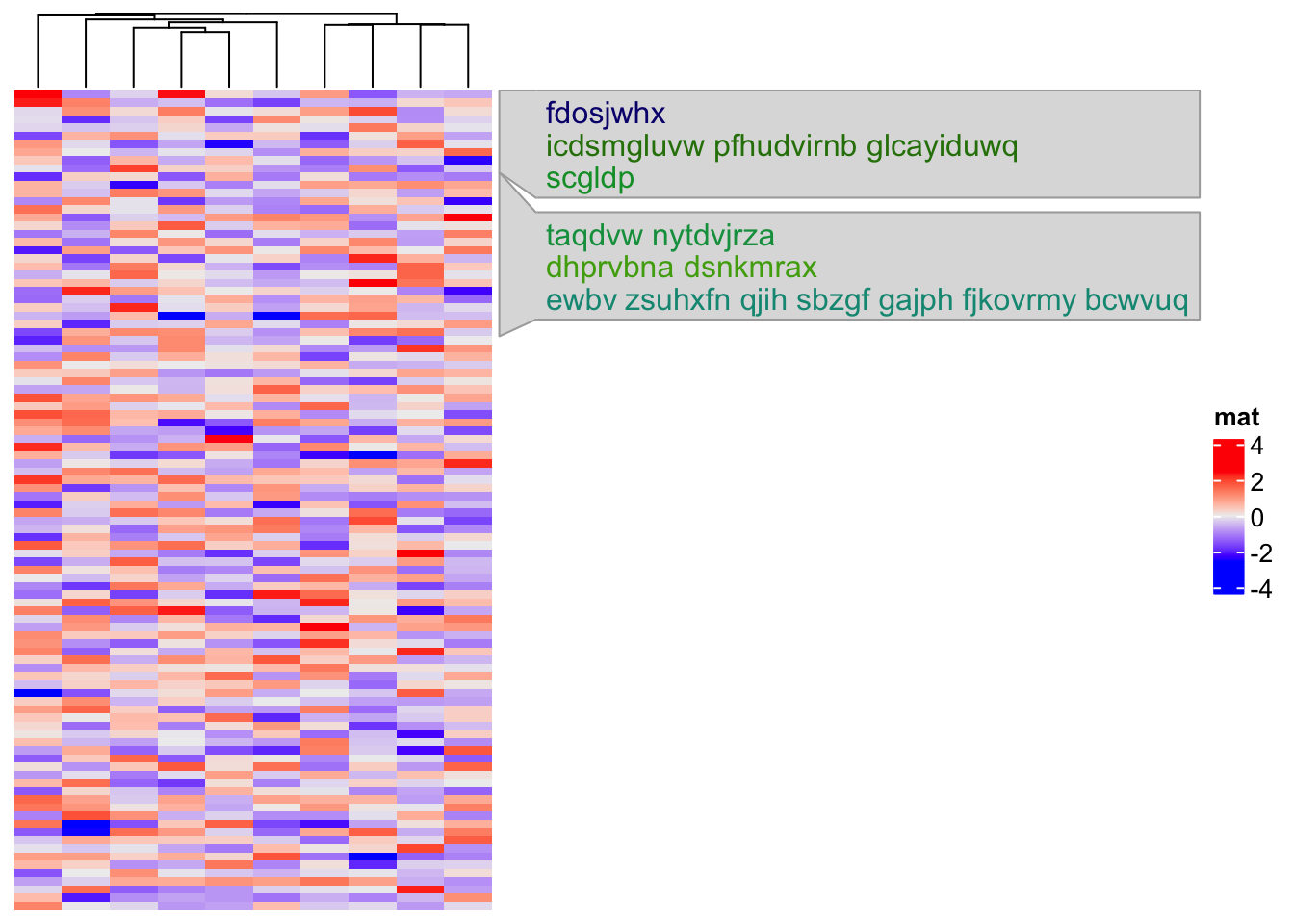
In following we show how to add a “complex version” of points annotation. The only thing that needs to be careful is the location on x-axis (y-axis if it is a row annotation) should correspond to the column index after column reordering.

# Note this example is only for demonstration of `anno_empty()`.
# Actually it can be made easily by `anno_points()`.
ha = HeatmapAnnotation(foo = anno_empty(border = TRUE, height = unit(3, "cm")))
ht = Heatmap(matrix(rnorm(100), nrow = 10), name = "mat", top_annotation = ha)
ht = draw(ht)
co = column_order(ht)
value = runif(10)
decorate_annotation("foo", {
    # value on x-axis is always 1:ncol(mat)
    x = 1:10
    # while values on y-axis is the value after column reordering
    value = value[co]
    pushViewport(viewport(xscale = c(0.5, 10.5), yscale = c(0, 1)))
    grid.lines(c(0.5, 10.5), c(0.5, 0.5), gp = gpar(lty = 2),
        default.units = "native")
    grid.points(x, value, pch = 16, size = unit(2, "mm"),
        gp = gpar(col = ifelse(value > 0.5, "red", "blue")), default.units = "native")
    grid.yaxis(at = c(0, 0.5, 1))
    popViewport()
})

3.4 Block annotation

There are two uses for block annotation. 1. simply as rectangles (with labels inside) to mark heatmap slices, 2. as plotting regions to associate subsets of rows or columns in the heatmap.

3.4.1 Block for putting labels

In this case, the block annotation is more like a color block which identifies groups when the rows or columns of the heatmap are split.

Heatmap(matrix(rnorm(100), 10), name = "mat",
    top_annotation = HeatmapAnnotation(foo = anno_block(gp = gpar(fill = 2:4))),
    column_km = 3)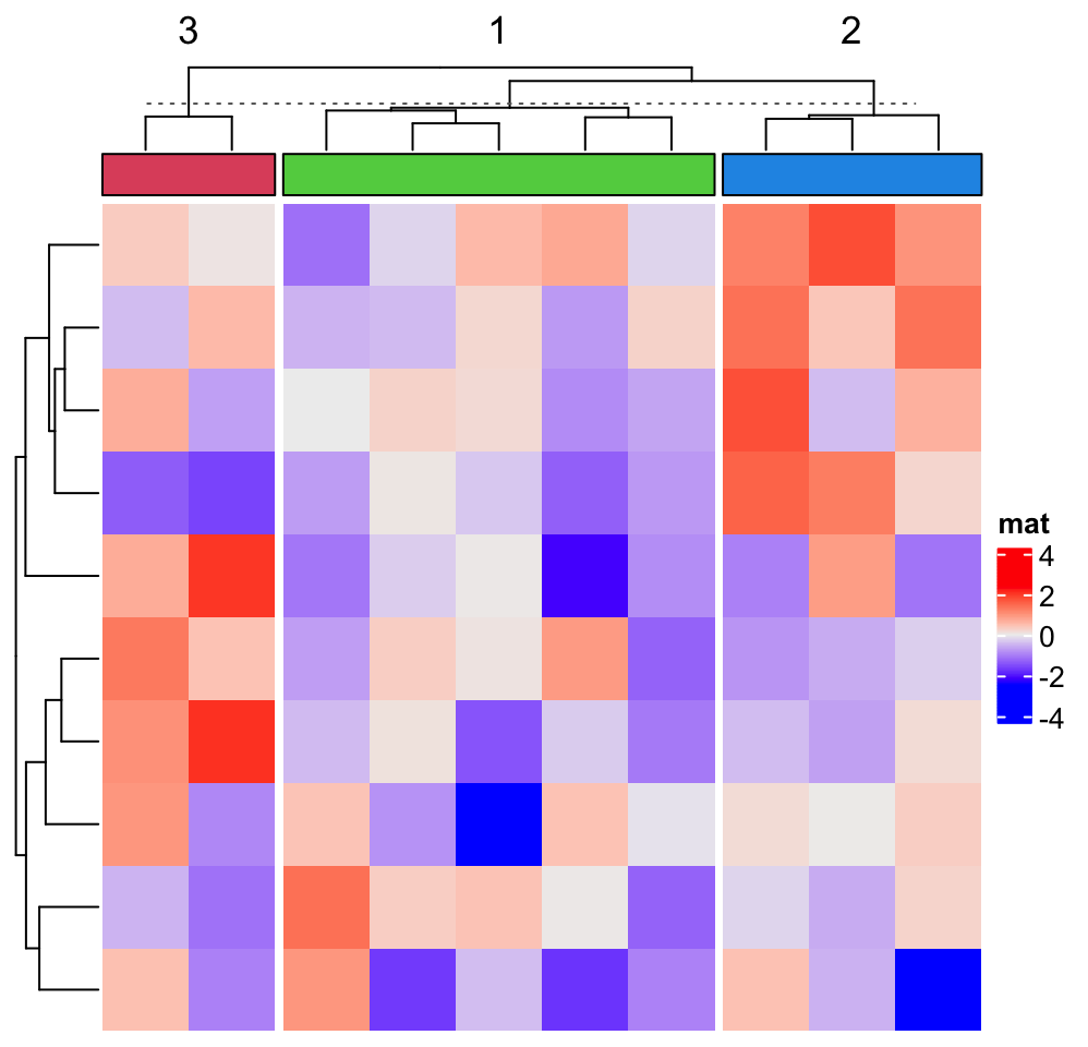

Labels can be added to each block.

Heatmap(matrix(rnorm(100), 10), name = "mat",
    top_annotation = HeatmapAnnotation(foo = anno_block(gp = gpar(fill = 2:4),
        labels = c("group1", "group2", "group3"), 
        labels_gp = gpar(col = "white", fontsize = 10))),
    column_km = 3,
    left_annotation = rowAnnotation(foo = anno_block(gp = gpar(fill = 2:4),
        labels = c("group1", "group2", "group3"), 
        labels_gp = gpar(col = "white", fontsize = 10))),
    row_km = 3)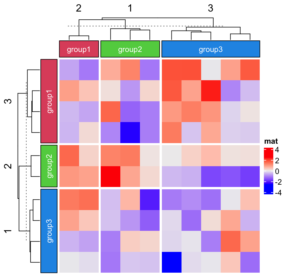

Note the length of labels or graphics parameters should have the same length as the number of slices.

anno_block() function draws rectangles for row/column slices where one rectangle only corresponds to one single slice. Then what if we want to draw the rectangles over several slices to show they belong to certain groups?

Currently, it is difficult to directly support it in anno_block(), however, there is workaround for it. Actually, to draw rectangles across several slices, we need to know two things: 1. the positions of the slices in the plot, and 2. space to draw the rectangles. Luckily, the positions can be obtained by directly go to the correspoding viewport and the space can be allocated by anno_empty() function.

In the following code, we use anno_empty() to create an empty annotation:

set.seed(123)
mat2 = matrix(rnorm(50*50), nrow = 50)
split = rep(1:5, each = 10)
ha = HeatmapAnnotation(
    empty = anno_empty(border = FALSE),
    foo = anno_block(gp = gpar(fill = 2:6), labels = LETTERS[1:5])
)
Heatmap(mat2, name = "mat2", column_split = split, top_annotation = ha, 
    column_title = NULL)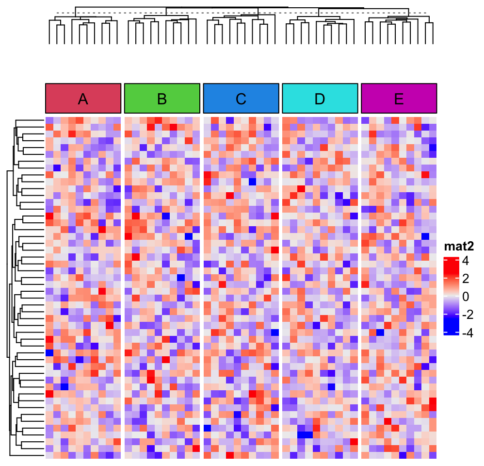

Let’s say, we want to put the first three column slices as a group and the last two slices as the second group.

The positions of the first and the third slices for annotation "empty" can be obtained by:

seekViewport("annotation_empty_1")
loc1 = deviceLoc(x = unit(0, "npc"), y = unit(0, "npc"))
seekViewport("annotation_empty_3")
loc2 = deviceLoc(x = unit(1, "npc"), y = unit(1, "npc"))
loc2

## $x
## [1] 4.07403126835173inches
## 
## $y
## [1] 6.51051067246731inches

The viewport name "annotation_empty_1" correspond to the first slice for annotation empty, and we take the left bottom of the first “empty” annotation slice and the top right of the third slice, saved in loc1 and loc2 variables.

Here what is important is the use of grid::deviceLoc() function. It directly converts a location measured in a certain viewport to the position in the graphics device.

In the end, we go to the "global" viewport because the size of "global" viewport is the size of the graphics device, and draw the rectangle and add label.

seekViewport("global")
grid.rect(loc1$x, loc1$y, width = loc2$x - loc1$x, height = loc2$y - loc1$y, 
    just = c("left", "bottom"), gp = gpar(fill = "red"))
grid.text("group 1", x = (loc1$x + loc2$x)*0.5, y = (loc1$y + loc2$y)*0.5)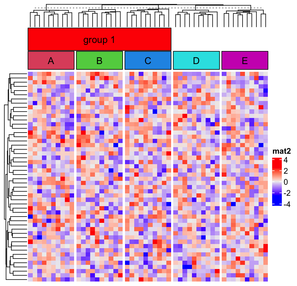

The viewport names for the annotations are in a fixed format, which is annotation_{annotation_name}_{slice_index}. The full set of viewport names can be obtained by list_components() function.

list_components()

##  [1] "ROOT"                        "global"                     
##  [3] "global_layout"               "global-heatmaplist"         
##  [5] "main_heatmap_list"           "heatmap_mat2"               
##  [7] "mat2_heatmap_body_wrap"      "mat2_heatmap_body_1_1"      
##  [9] "mat2_heatmap_body_1_2"       "mat2_heatmap_body_1_3"      
## [11] "mat2_heatmap_body_1_4"       "mat2_heatmap_body_1_5"      
## [13] "mat2_dend_row_1"             "mat2_dend_column_1"         
## [15] "mat2_dend_column_2"          "mat2_dend_column_3"         
## [17] "mat2_dend_column_4"          "mat2_dend_column_5"         
## [19] "annotation_empty_1"          "annotation_foo_1"           
## [21] "annotation_empty_2"          "annotation_foo_2"           
## [23] "annotation_empty_3"          "annotation_foo_3"           
## [25] "annotation_empty_4"          "annotation_foo_4"           
## [27] "annotation_empty_5"          "annotation_foo_5"           
## [29] "global-heatmap_legend_right" "heatmap_legend"

If more than one group-level rectangles are to be added, we can wrap the code into a simple function group_block_anno():

ha = HeatmapAnnotation(
    empty = anno_empty(border = FALSE, height = unit(8, "mm")),
    foo = anno_block(gp = gpar(fill = 2:6), labels = LETTERS[1:5])
)
Heatmap(mat2, name = "mat2", column_split = split, top_annotation = ha, 
    column_title = NULL)

library(GetoptLong)  # for the function qq()
group_block_anno = function(group, empty_anno, gp = gpar(), 
    label = NULL, label_gp = gpar()) {

    seekViewport(qq("annotation_@{empty_anno}_@{min(group)}"))
    loc1 = deviceLoc(x = unit(0, "npc"), y = unit(0, "npc"))
    seekViewport(qq("annotation_@{empty_anno}_@{max(group)}"))
    loc2 = deviceLoc(x = unit(1, "npc"), y = unit(1, "npc"))

    seekViewport("global")
    grid.rect(loc1$x, loc1$y, width = loc2$x - loc1$x, height = loc2$y - loc1$y, 
        just = c("left", "bottom"), gp = gp)
    if(!is.null(label)) {
        grid.text(label, x = (loc1$x + loc2$x)*0.5, y = (loc1$y + loc2$y)*0.5, gp = label_gp)
    }
}

group_block_anno(1:3, "empty", gp = gpar(fill = "red"), label = "group 1")
group_block_anno(4:5, "empty", gp = gpar(fill = "blue"), label = "group 2")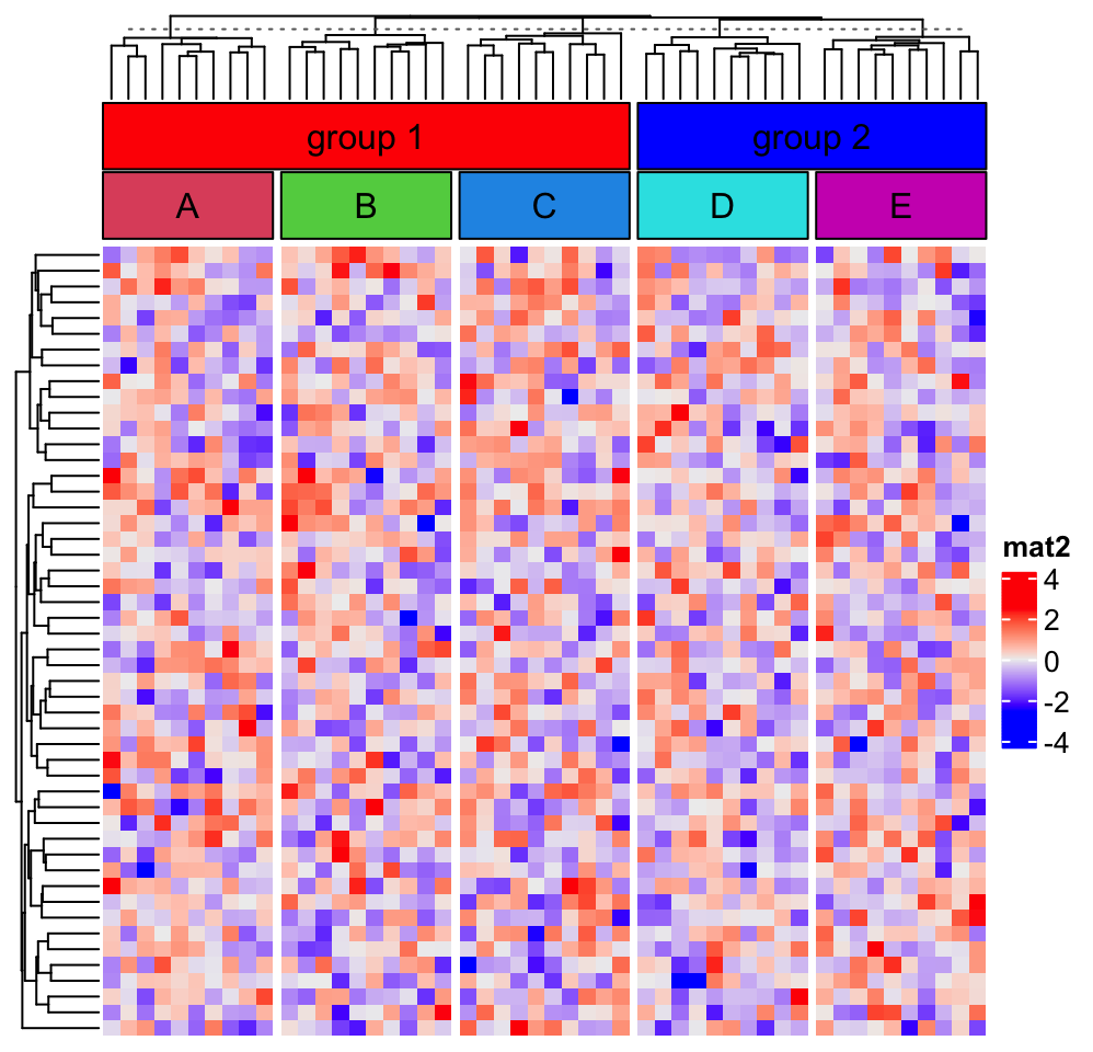

3.4.2 Blocks as plotting regions

When heatmap is split, each block in block annotation can be thought as a virtual plotting region. anno_block() allows an argument panel_fun which accepts a self-defined function that draws graphics in each slice. It must have two arguments:

1. row/column indices for the current slice (let’s call it index),
2. a vector of levels from the split variable that correspond to current slice (let’s call it level). When e.g. row_km is only set or row_split is only set to one categorical variable, then level is a vector of length one. If there are multiple categorical variables set with row_km and row_split, level is a vector of which the length is the same as the number of categorical variables.

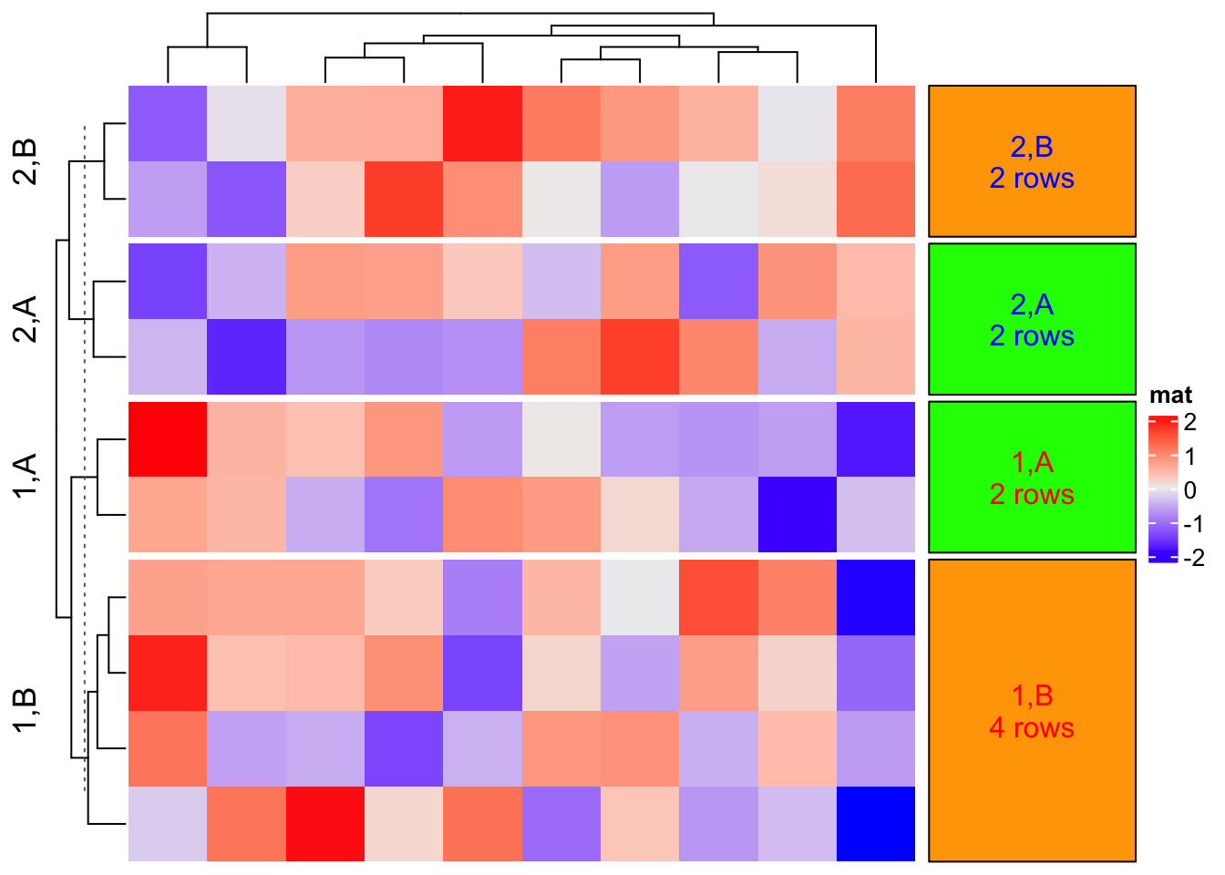
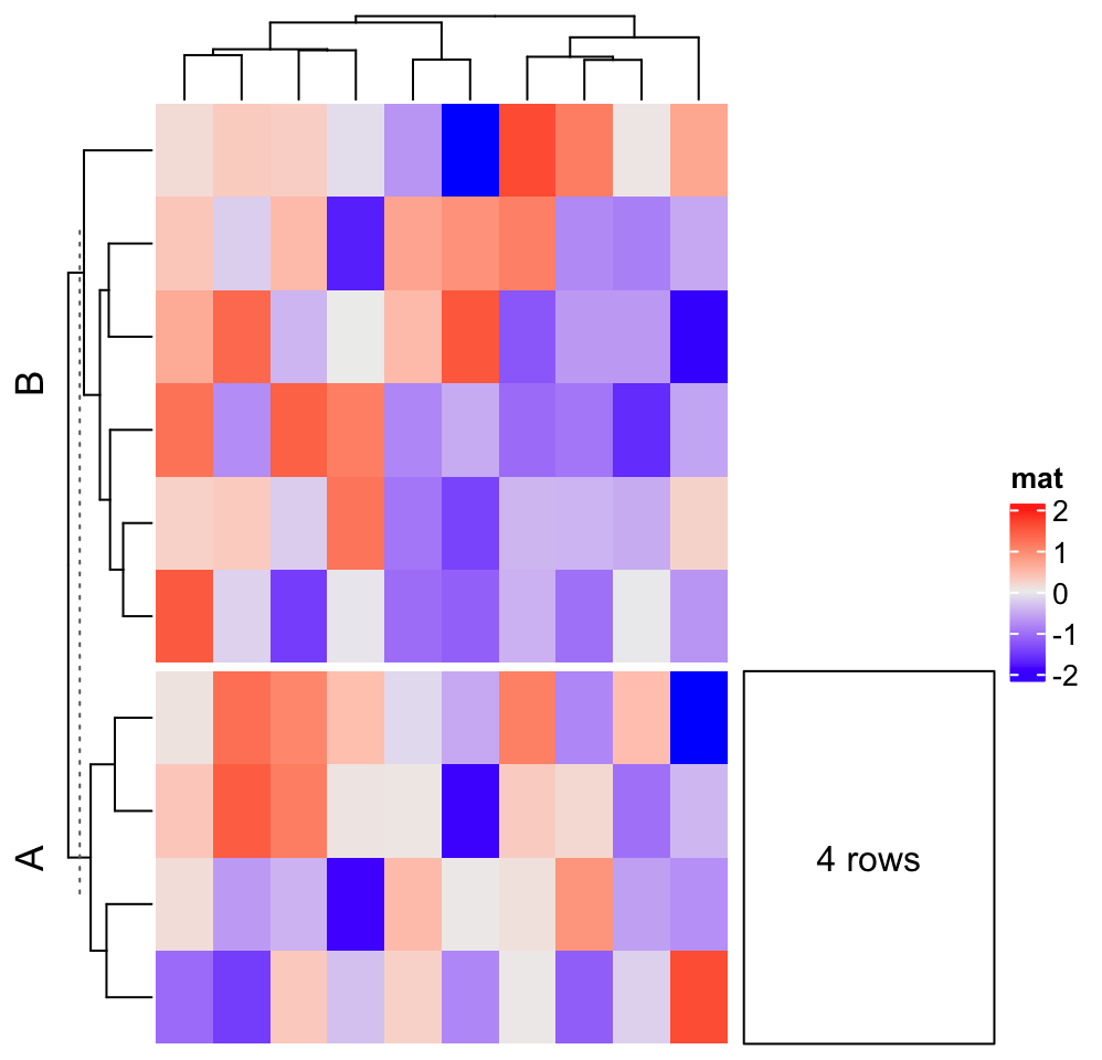
When panel_fun is set, all other graphics parameters in anno_block() are ignored. See the following example:

col = c("1" = "red", "2" = "blue", "A" = "green", "B" = "orange")
Heatmap(matrix(rnorm(100), 10), name = "mat", row_km = 2, 
    row_split = sample(c("A", "B"), 10, replace = TRUE)) + 
rowAnnotation(foo = anno_block(
    panel_fun = function(index, levels) {
        grid.rect(gp = gpar(fill = col[levels[2]], col = "black"))
        txt = paste(levels, collapse = ",")
        txt = paste0(txt, "\n", length(index), " rows")
        grid.text(txt, 0.5, 0.5, rot = 0,
            gp = gpar(col = col[levels[1]]))
    },
    width = unit(3, "cm")
))

To make it more general, anno_block() accepts an argument align_to which defines a list of indices that blocks will be corresponded to, but you need to make sure the indices are continuously adjacent on heatmaps.

split = sample(c("A", "B"), 10, replace = TRUE)
align_to = list("A" = which(split == "A"))
panel_fun = function(index, nm) {
    grid.rect()
    grid.text(paste0(length(index), " rows"), 0.5, 0.5)
}
Heatmap(matrix(rnorm(100), 10), name = "mat", row_split = split) + 
rowAnnotation(foo = anno_block(
    align_to = align_to,
    panel_fun = panel_fun,
    width = unit(3, "cm")
))

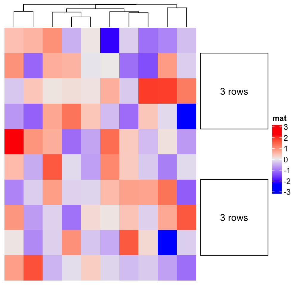
anno_block() normally works with row_split, but it is not necessary, see the following example:

align_to = list("A" = 2:4, "B" = 7:9)
Heatmap(matrix(rnorm(100), 10), name = "mat", cluster_rows = FALSE) + 
rowAnnotation(foo = anno_block(
    align_to = align_to,
    panel_fun = panel_fun,
    width = unit(3, "cm")
))

3.5 Image annotation

Images can be added as annotations. anno_image() supports image in png, svg, pdf, eps, jpeg/jpg, tiff formats. How they are imported as annotations are as follows:

• png, jpeg/jpg and tiff images are imported by png::readPNG(), jpeg::readJPEG() and tiff::readTIFF(), and drawn by grid::grid.raster().
• svg images are firstly reformatted by rsvg::rsvg_svg() and then imported by grImport2::readPicture() and drawn by grImport2::grid.picture().
• pdf and eps images are imported by grImport::PostScriptTrace() and grImport::readPicture(), later drawn by grImport::grid.picture().

The free icons for following examples are from https://github.com/Keyamoon/IcoMoon-Free. A vector of image paths are set as the first argument of anno_image().

image_png = sample(dir("IcoMoon-Free-master/PNG/64px", full.names = TRUE), 10)
image_svg = sample(dir("IcoMoon-Free-master/SVG/", full.names = TRUE), 10)
image_eps = sample(dir("IcoMoon-Free-master/EPS/", full.names = TRUE), 10)
image_pdf = sample(dir("IcoMoon-Free-master/PDF/", full.names = TRUE), 10)

# we only draw the image annotation for PNG images, while the others are the same
ha = HeatmapAnnotation(foo = anno_image(image_png))

Different image formats can be mixed in the input vector.

# code only for demonstration
ha = HeatmapAnnotation(foo = anno_image(c(image_png[1:3], image_svg[1:3], 
    image_eps[1:3], image_pdf[1:3])))

Border and background colors (if the images have transparent background) can be set by gp.

ha = HeatmapAnnotation(foo = anno_image(image_png, 
    gp = gpar(fill = 1:10, col = "black")))

border controls the border of the whole annotation.

ha = HeatmapAnnotation(foo = anno_image(image_png, border = "red"))

Padding or space around the images is set by space.

ha = HeatmapAnnotation(foo = anno_image(image_png, space = unit(3, "mm")))

If only some of the images need to be drawn, the other elements in the image vector can be set to '' or NA.

image_png[1:2] = ""
ha = HeatmapAnnotation(foo = anno_image(image_png))

3.6 Points annotation

Points annotation implemented by anno_points() shows distribution of a list of data points. The data points object x can be a single vector or a matrix. If it is a matrix, the graphics settings such as pch, size and gp can correpspond to matrix columns. Note again, if x is a matrix, rows in x correspond to columns in the heatmap matrix.

ha = HeatmapAnnotation(foo = anno_points(runif(10)))

ha = HeatmapAnnotation(foo = anno_points(matrix(runif(20), nc = 2), 
    pch = 1:2, gp = gpar(col = 2:3)))

ylim controls the range on “y-axis” or the “data axis” (if it is a row annotation, the data axis is horizontal), extend controls the extended space on the data axis direction. axis controls whether to show the axis and axis_param controls the settings for axis. The default settings for axis are:

default_axis_param("column")

## $at
## NULL
## 
## $labels
## NULL
## 
## $labels_rot
## [1] 0
## 
## $gp
## $fontsize
## [1] 8
## 
## 
## $side
## [1] "left"
## 
## $facing
## [1] "outside"
## 
## $direction
## [1] "normal"

And you can overwrite some of them:

ha = HeatmapAnnotation(foo = anno_points(runif(10), ylim = c(0, 1),
    axis_param = list(
        side = "right",
        at = c(0, 0.5, 1), 
        labels = c("zero", "half", "one")
    ))
)

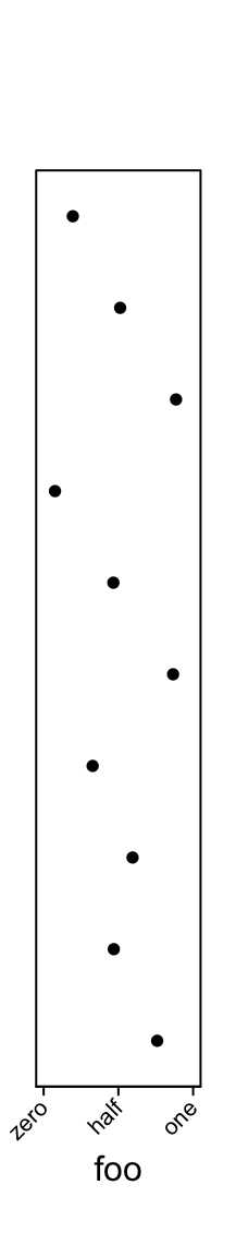
One thing that might be useful is you can control the rotation of the axis labels.

ha = rowAnnotation(foo = anno_points(runif(10), ylim = c(0, 1),
    width = unit(2, "cm"),
    axis_param = list(
        side = "bottom",
        at = c(0, 0.5, 1), 
        labels = c("zero", "half", "one"),
        labels_rot = 45
    ))
)

The configuration of axis is same for all other annotation functions which have axes.

The default size of the points annotation is 5mm. It can be controlled by height/width argument in anno_points().

ha = HeatmapAnnotation(foo = anno_points(runif(10), height = unit(2, "cm")))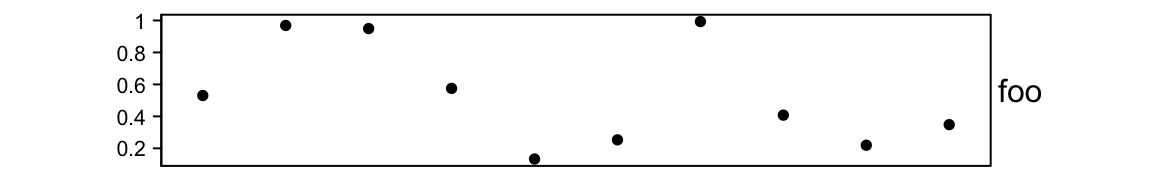

3.7 Line annotation

anno_lines() connects the data points by a list of segments. Similar as anno_points(), the data variable can be a numeric vector:

ha = HeatmapAnnotation(foo = anno_lines(runif(10)))

Or a matrix:

ha = HeatmapAnnotation(foo = anno_lines(cbind(c(1:5, 1:5), c(5:1, 5:1)), 
    gp = gpar(col = 2:3), add_points = TRUE, pt_gp = gpar(col = 5:6), pch = c(1, 16)))

As shown above, points can be added to the lines by setting add_points = TRUE.

Smoothed lines (by loess()) can be added instead of the original lines by setting smooth = TRUE, but it should be used with caution because the order of columns in the heatmap is used as “x-value” for the fitting and only if you think the fitting against the reordered order makes sense.

Smoothing also works when the input data variable is a matrix that the smoothing is performed for each column separately.

If smooth is TRUE, add_points is set to TRUE by default.

ha = HeatmapAnnotation(foo = anno_lines(runif(10), smooth = TRUE))

The default size of the lines annotation is 5mm. It can be controlled by height/width argument in anno_lines().

# code only for demonstration
ha = HeatmapAnnotation(foo = anno_lines(runif(10), height = unit(2, "cm")))

3.8 Barplot annotation

The data points can be represented as barplots. Some of the arguments in anno_barplot() such as ylim, axis, axis_param are the same as anno_points().

ha = HeatmapAnnotation(foo = anno_barplot(1:10))

The width of bars is controlled by bar_width. It is a relative value to the width of the cell in the heatmap.

ha = HeatmapAnnotation(foo = anno_barplot(1:10, bar_width = 1))

Graphic parameters are controlled by gp.

ha = HeatmapAnnotation(foo = anno_barplot(1:10, gp = gpar(fill = 1:10)))

You can choose the baseline of bars by baseline.

ha = HeatmapAnnotation(foo = anno_barplot(seq(-5, 5), baseline = "min"))

ha = HeatmapAnnotation(foo = anno_barplot(seq(-5, 5), baseline = 0))

If the input value is a matrix, it will be stacked barplots.

ha = HeatmapAnnotation(foo = anno_barplot(matrix(nc = 2, c(1:10, 10:1))))

And length of parameters in gp can be the number of the columns in the matrix:

ha = HeatmapAnnotation(foo = anno_barplot(cbind(1:10, 10:1), 
    gp = gpar(fill = 2:3, col = 2:3)))

The default size of the barplot annotation is 5mm. It can be controlled by height/width argument in anno_barplot().

# code only for demonstration
ha = HeatmapAnnotation(foo = anno_barplot(runif(10), height = unit(2, "cm")))

Following example shows a barplot annotation which visualizes a proportion matrix (for which row sums are 1).

m = matrix(runif(4*10), nc = 4)
m = t(apply(m, 1, function(x) x/sum(x)))
ha = HeatmapAnnotation(foo = anno_barplot(m, gp = gpar(fill = 2:5), 
    bar_width = 1, height = unit(6, "cm")))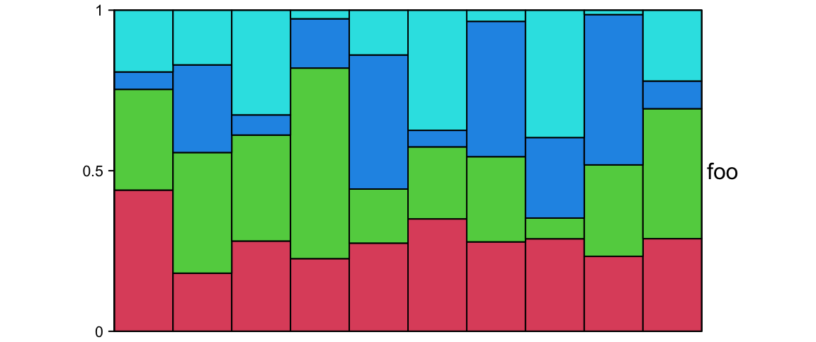

The direction of the axis can be reversed which is useful when the annotation is put on the left of the heatmap.

ha_list = rowAnnotation(axis_reverse = anno_barplot(m, gp = gpar(fill = 2:5), 
    axis_param = list(direction = "reverse"), 
    bar_width = 1, width = unit(4, "cm"))) +
rowAnnotation(axis_normal = anno_barplot(m, gp = gpar(fill = 2:5), 
    bar_width = 1, width = unit(4, "cm")))
draw(ha_list, ht_gap = unit(4, "mm"))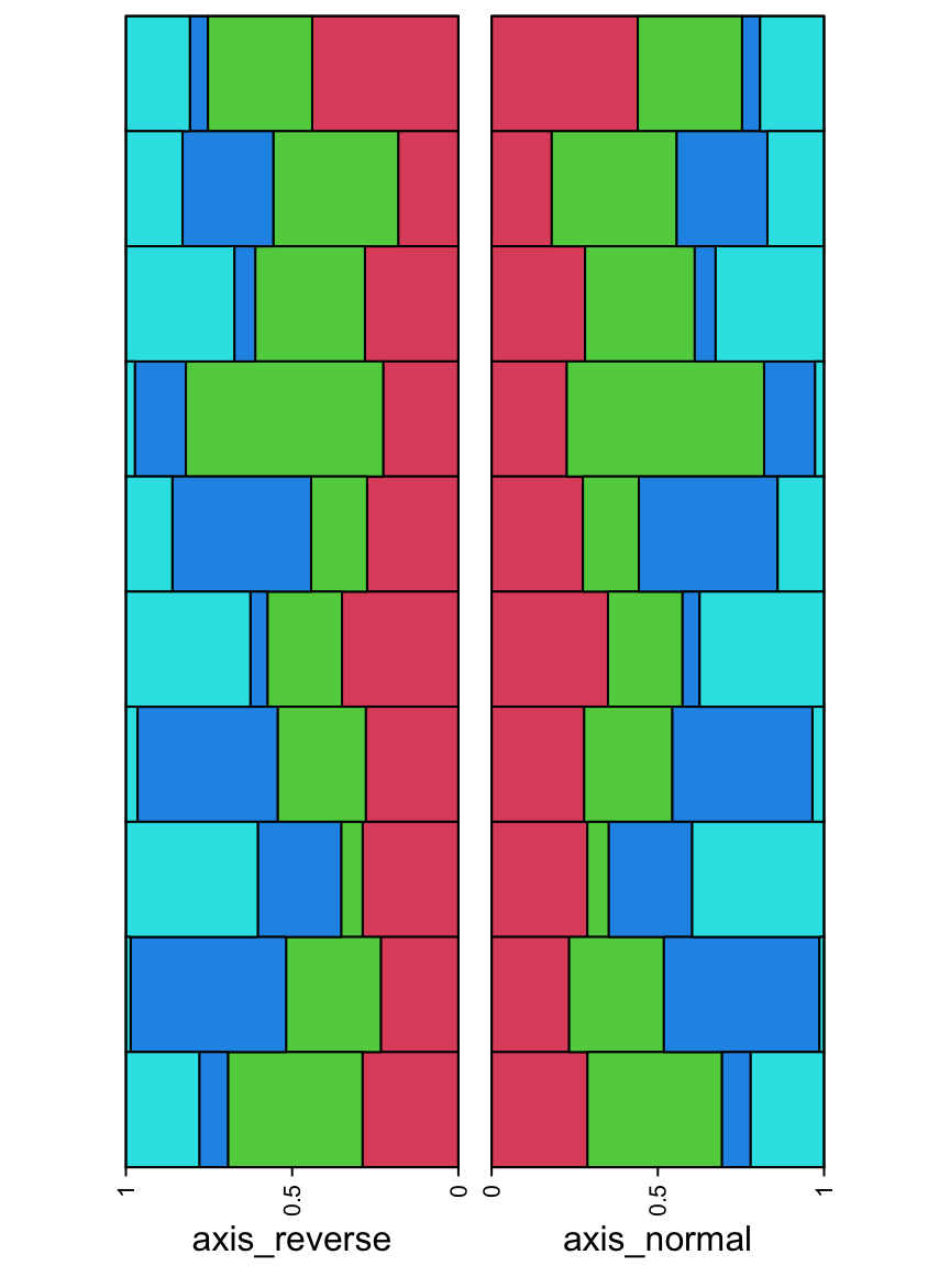

direction = "reverse" also works for other annotation functions which have axes, but it is more commonly used for barplot annotations.

Argument add_numbers can be set to TRUE so that numbers associated to bars are drawn on top of the bars. For column annotation, texts are by default with 45 degree rotation.

ha = HeatmapAnnotation(foo = anno_barplot(1:10, add_numbers = TRUE, 
    height = unit(1, "cm")))

When the input for anno_barplot() is a matrix, argument beside can be set to TRUE so that bars for a same heatmap column are positioned by each other:

ha = HeatmapAnnotation(foo = anno_barplot(matrix(nc = 2, c(1:10, 10:1)), 
    beside = TRUE))

Argument attach can be set to TRUE so that two adjacent bars are attached.

ha = HeatmapAnnotation(foo = anno_barplot(matrix(nc = 2, c(1:10, 10:1)), 
    beside = TRUE, attach = TRUE))

3.9 Boxplot annotation

Boxplot annotation as well as the annotation functions which are introduced later are more suitable for small matrice. I don’t think you want to put boxplots as column annotation for a matrix with 100 columns.

For anno_boxplot(), the input data variable should be a matrix or a list. If x is a matrix and if it is a column annotation, statistics for boxplots are calculated by columns, and if it is a row annotation, the calculation is done by rows.

set.seed(12345)
m = matrix(rnorm(100), 10)
ha = HeatmapAnnotation(foo = anno_boxplot(m, height = unit(4, "cm")))

Graphic parameters are controlled by gp.

ha = HeatmapAnnotation(foo = anno_boxplot(m, height = unit(4, "cm"), 
    gp = gpar(fill = 1:10)))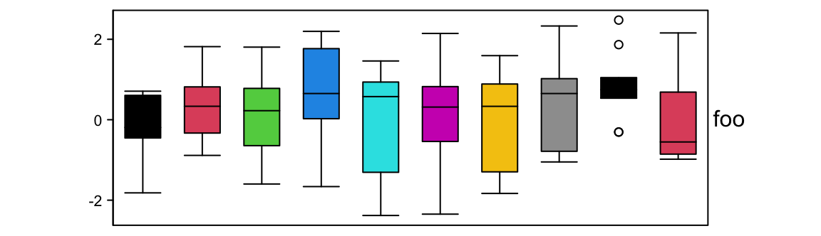

Width of the boxes are controlled by box_width. outline controls whether to show outlier points.

ha = HeatmapAnnotation(foo = anno_boxplot(m, height = unit(4, "cm"), 
    box_width = 0.9, outline = FALSE))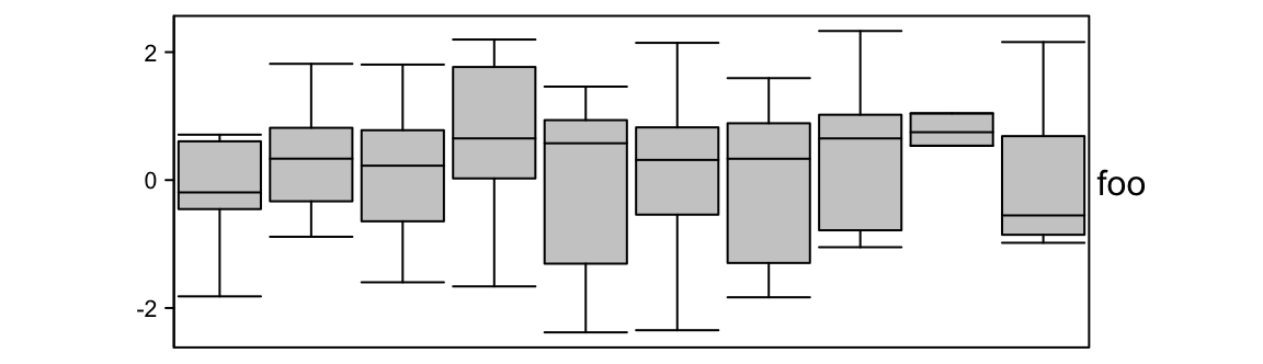

anno_boxplot() only draws one boxplot for one single row. Section 14.6 demonstrates how to define an annotation function which draws multiple boxplots for a single row, and Section 3.18 demonstrates how to draw one single boxplot for a group of rows.

3.10 Histogram annotation

Annotations as histograms are more suitable to put as row annotations. The setting for the data variable is the same as anno_boxplot() which can be a matrix or a list.

Similar as anno_boxplot(), the input data variable should be a matrix or a list. If x is a matrix and if it is a column annotation, histograms are calculated by columns, and if it is a row annotation, histograms are calculated by rows.

m = matrix(rnorm(1000), nc = 100)
ha = rowAnnotation(foo = anno_histogram(m)) # apply `m` on rows

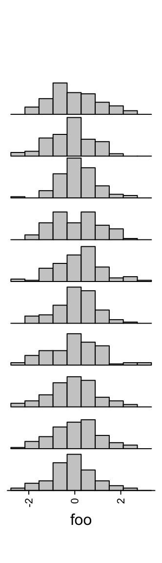
Number of breaks for histograms is controlled by n_breaks.

ha = rowAnnotation(foo = anno_histogram(m, n_breaks = 20))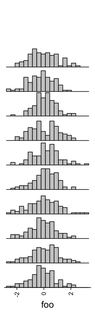

Colors are controlled by gp.

ha = rowAnnotation(foo = anno_histogram(m, gp = gpar(fill = 1:10)))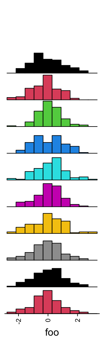

3.11 Density annotation

Similar as histogram annotations, anno_density() shows the distribution as a fitted curve.

ha = rowAnnotation(foo = anno_density(m))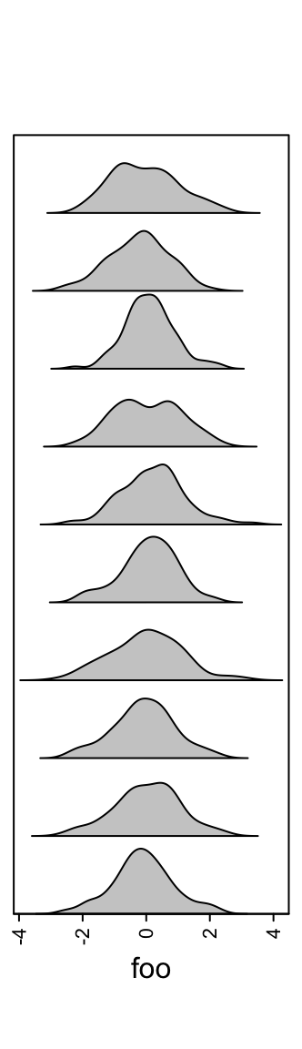

The height of the density peaks can be controlled to make the distribution look like a “joyplot”.

ha = rowAnnotation(foo = anno_density(m, joyplot_scale = 2, 
    gp = gpar(fill = "#CCCCCC80")))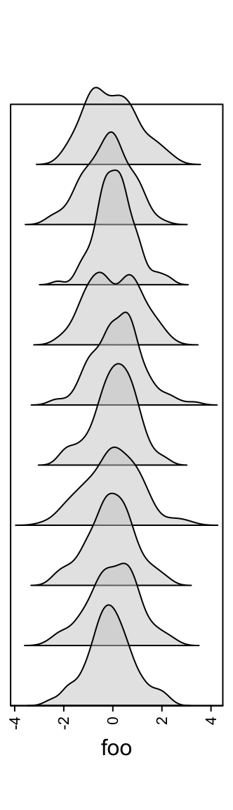

Or visualize the distribution as violin plot.

ha = rowAnnotation(foo = anno_density(m, type = "violin", 
    gp = gpar(fill = 1:10)))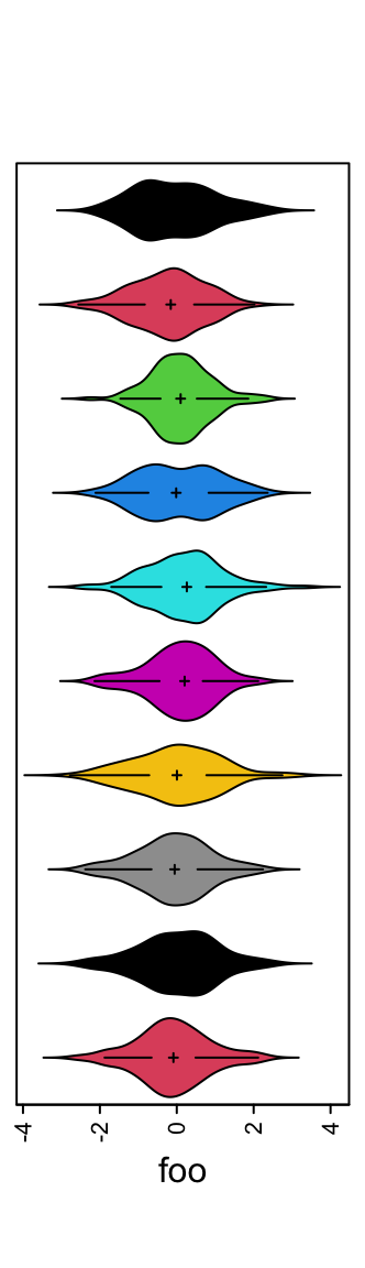

When there are too many rows in the input variable, the space for normal density peaks might be too small. In this case, we can visualize the distribution by heatmaps.

m2 = matrix(rnorm(50*10), nrow = 50)
ha = rowAnnotation(foo = anno_density(m2, type = "heatmap", width = unit(6, "cm")))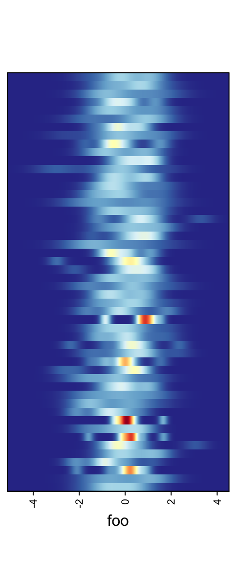

THe color schema for heatmap distribution is controlled by heatmap_colors.

ha = rowAnnotation(foo = anno_density(m2, type = "heatmap", width = unit(6, "cm"), 
    heatmap_colors = c("white", "orange")))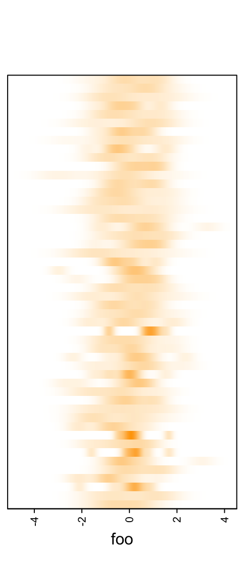

In ComplexHeatmap package, there is a densityHeatmap() function which visualizes distribution as a heatmap. It will be introduced in Section 11.1.

3.12 Joyplot annotation

anno_joyplot() is specific for so-called joyplot (http://blog.revolutionanalytics.com/2017/07/joyplots.html). The input data should be a matrix or a list.

Note anno_joyplot() is always applied to columns if the input is a matrix. Because joyplot visualizes parallel distributions and the matrix is not a necessary format while a list is already enough for it, if you are not sure about how to set as a matrix, just convert it to a list for using it.

m = matrix(rnorm(1000), nc = 10)
lt = apply(m, 2, function(x) data.frame(density(x)[c("x", "y")]))
ha = rowAnnotation(foo = anno_joyplot(lt, width = unit(4, "cm"), 
    gp = gpar(fill = 1:10), transparency = 0.75))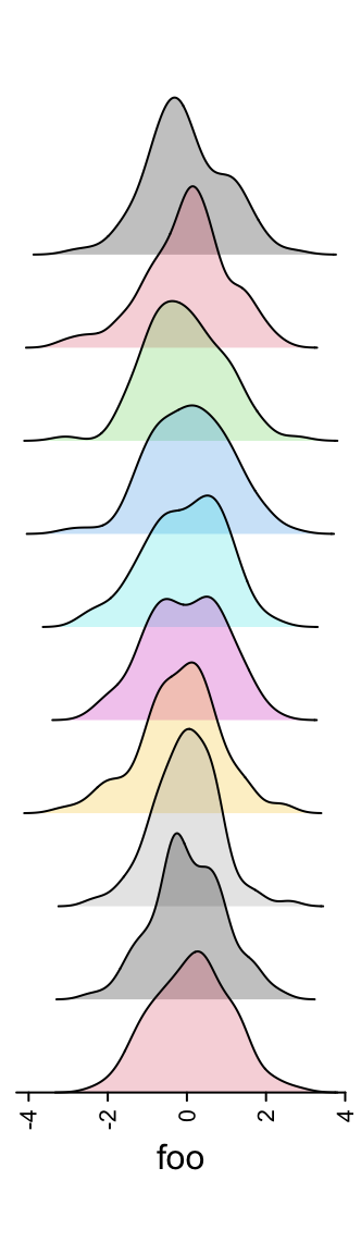

Or only show the lines (scale argument controls the relative height of the curves).

m = matrix(rnorm(5000), nc = 50)
lt = apply(m, 2, function(x) data.frame(density(x)[c("x", "y")]))
ha = rowAnnotation(foo = anno_joyplot(lt, width = unit(4, "cm"), gp = gpar(fill = NA), 
    scale = 4))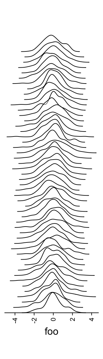

The format of the input variable is special. It can be one of the following two:

1. a matrix (remember anno_joyplot() is always applied to columns of the matrix) where x coordinate corresponds to 1:nrow(matrix) and each column in the matrix corresponds to one distribution in the joyplot.
2. a list of data frames where each data frame has two columns which correspond to x coordinate and y coordinate.

3.13 Horizon chart annotation

Horizon chart as annotation can only be added as row annotation. The format of the input variable for anno_horizon() is the same as anno_joyplot() which is introduced in previous section.

The default style of horizon chart annotation is:

lt = lapply(1:20, function(x) cumprod(1 + runif(1000, -x/100, x/100)) - 1)
ha = rowAnnotation(foo = anno_horizon(lt))

Values in each track are normalized by x/max(abs(x)).

Colors for positive values and negative values are controlled by pos_fill and neg_fill in gpar().

ha = rowAnnotation(foo = anno_horizon(lt, 
    gp = gpar(pos_fill = "orange", neg_fill = "darkgreen")))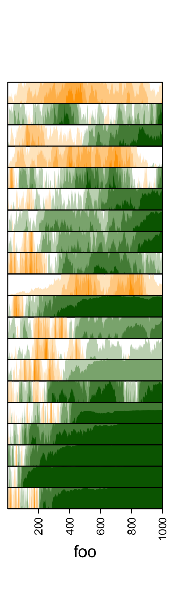

pos_fill and neg_fill can be assigned as a vector.

ha = rowAnnotation(foo = anno_horizon(lt, 
    gp = gpar(pos_fill = rep(c("orange", "red"), each = 10),
              neg_fill = rep(c("darkgreen", "blue"), each = 10))))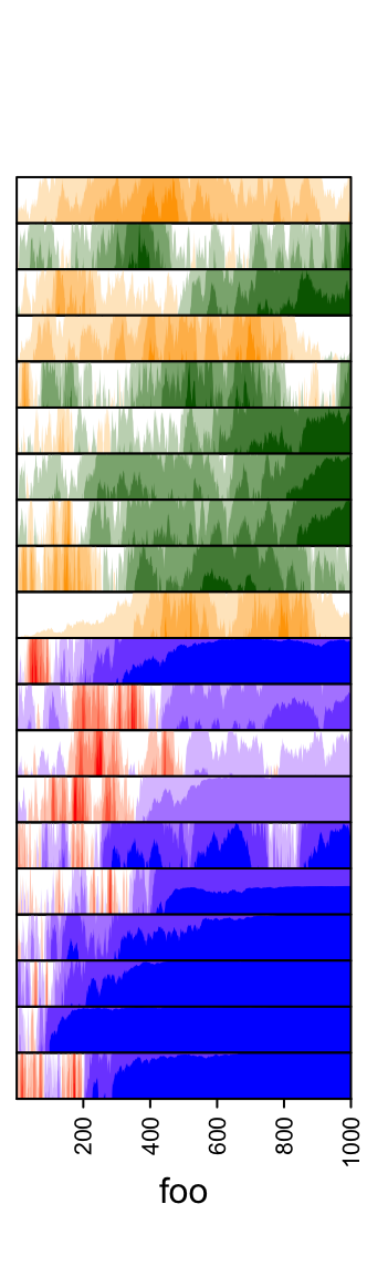

Whether the peaks for negative values start from the bottom or from the top.

ha = rowAnnotation(foo = anno_horizon(lt, negative_from_top = TRUE))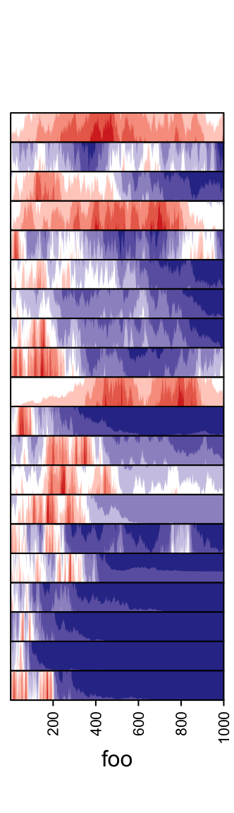

The space between every two neighbouring charts.

ha = rowAnnotation(foo = anno_horizon(lt, gap = unit(1, "mm")))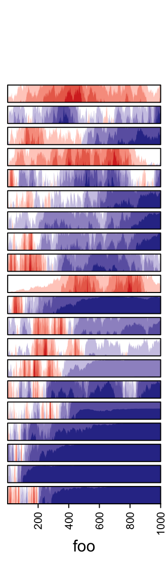

3.14 Text annotation

Text can be used as annotations by anno_text(). Graphics parameters are controlled by gp.

ha = rowAnnotation(foo = anno_text(month.name, gp = gpar(fontsize = 1:12+4)))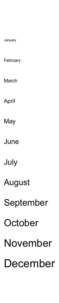

Locationsn are controlled by location and just. Rotation is controlled by rot.

ha = rowAnnotation(foo = anno_text(month.name, location = 1, rot = 30, 
    just = "right", gp = gpar(fontsize = 1:12+4)))

ha = rowAnnotation(foo = anno_text(month.name, location = 0.5, just = "center"))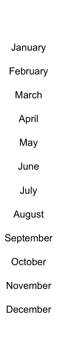

location and just are automatically calculated according the the position of the annotations put to the heatmap (e.g. text are aligned to the left if it is a right annotation to the heatmap and are aligned to the right it it is a left annotation).

The width/height are automatically calculated based on all the text. Normally you don’t need to manually set the width/height of it.

Background colors can be set by gp. Here fill controls the filled background color, col controls the color of text and the non-standard border controls the background border color.

You can see we explicitly set width as 1.2 times the width of the longest text.

ha = rowAnnotation(foo = anno_text(month.name, location = 0.5, just = "center",
    gp = gpar(fill = rep(2:4, each = 4), col = "white", border = "black"),
    width = max_text_width(month.name)*1.2))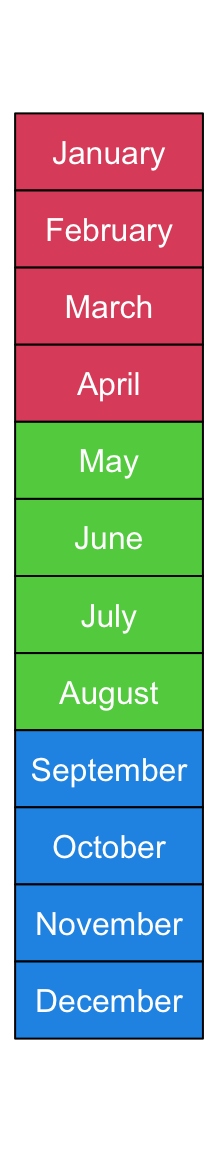

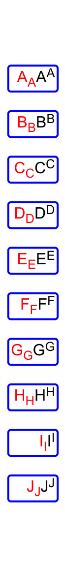
More complicated texts can be drawn by integrating with the gridtext package (Section 10.3.3). A quick example is as follows:

text = sapply(LETTERS[1:10], function(x) {
    qq("<span style='color:red'>**@{x}**<sub>@{x}</sub></span>_@{x}_<sup>@{x}</sup>")
})
ha = rowAnnotation(
    foo = anno_text(gt_render(text, align_widths = TRUE, 
                        r = unit(2, "pt"),
                        padding = unit(c(2, 2, 2, 2), "pt")), 
                    gp = gpar(box_col = "blue", box_lwd = 2), 
                    just = "right", 
                    location = unit(1, "npc")
    ))

Unlike other annotations, by default there is no annotation title for text annotation. The title can be added by setting show_name = TRUE in anno_text():

m = matrix(rnorm(100), 10)
Heatmap(m) + rowAnnotation(month = anno_text(month.name[1:10], just = "center", 
        location = unit(0.5, "npc"), show_name = TRUE), 
    annotation_name_rot = 0)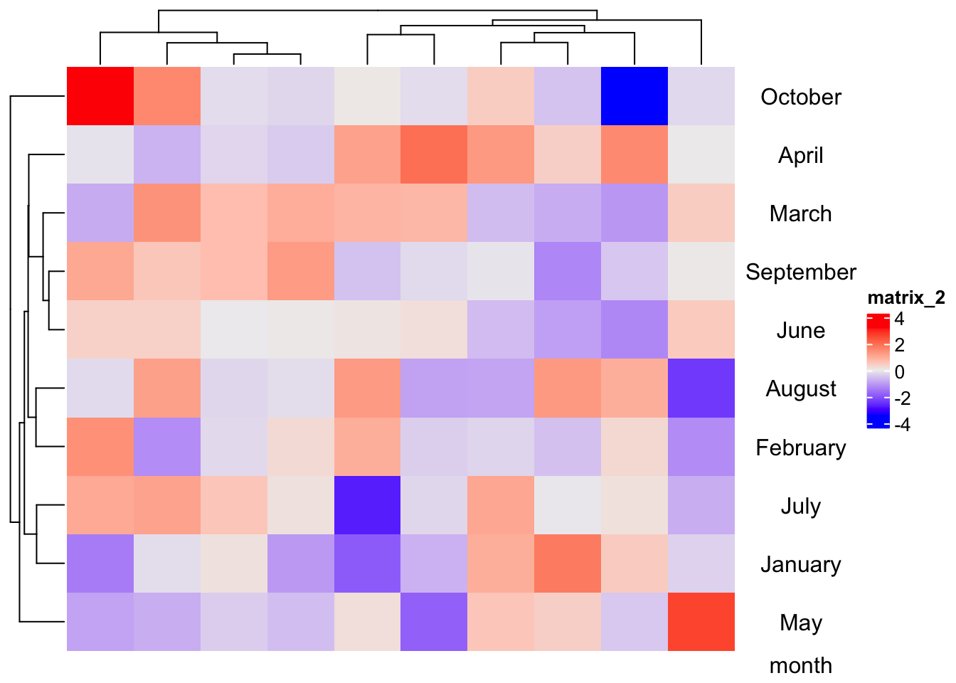

3.15 Numeric labels annotation

There is a special text annotation for numeric labels. To emphasize the visual effect, we also want to add bars to show the absolute values of the numbers. This can be done with anno_numeric() function. Note currently it only supports row annotation.

x = round(runif(10), 3)
ha = rowAnnotation(numeric = anno_numeric(x), annotation_name_rot = 0)

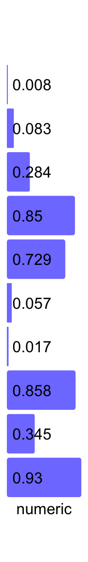
Background colors can by controlled by bg_gp.

ha = rowAnnotation(numeric = anno_numeric(x, 
        bg_gp = gpar(fill = "orange", col = "black")),
    annotation_name_rot = 0)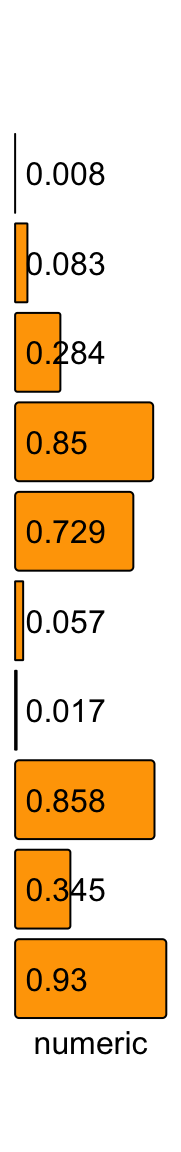

align_to can be set to "right" or "left":

ha = rowAnnotation(numeric = anno_numeric(x, 
        bg_gp = gpar(fill = "orange", col = "black"),
        align_to = "right"),
    annotation_name_rot = 0)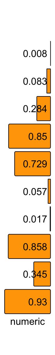

Format of labels on the plot can be controlled by labels_format:

ha = rowAnnotation(numeric = anno_numeric(x,
        labels_format = function(x) paste0(sprintf("%.2f", x*100), "%")),
    annotation_name_rot = 0)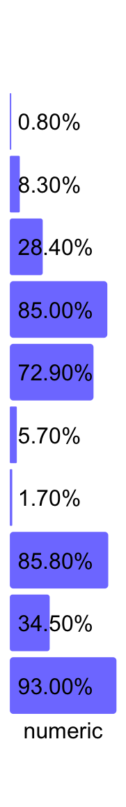

It is also possible to show a numeric vector with both negative and positive values. In this case, all graphics parameters should have length of two where the first one controls negative values and the second controls positive values.

x = round(runif(10, -1, 1), 3)
ha = rowAnnotation(numeric = anno_numeric(x, 
        bg_gp = gpar(fill = c("green", "red"))), 
    annotation_name_rot = 0)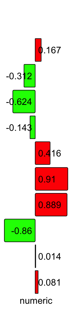

Another example is to visualize a vector of p-values. Here we should apply -log10() on p-values for mapping to bar heights with x_convert argument:

x = 10^(-runif(10, 1, 6))
ha = rowAnnotation(pvalue = anno_numeric(x, 
        rg = c(min(x), 1),
        x_convert = function(x) -log10(x), 
        labels_format = function(x) sprintf("%.2e", x)),
    annotation_name_rot = 0)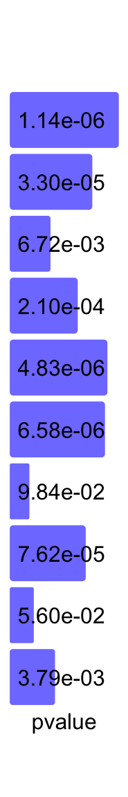

3.16 Completely customized annotation

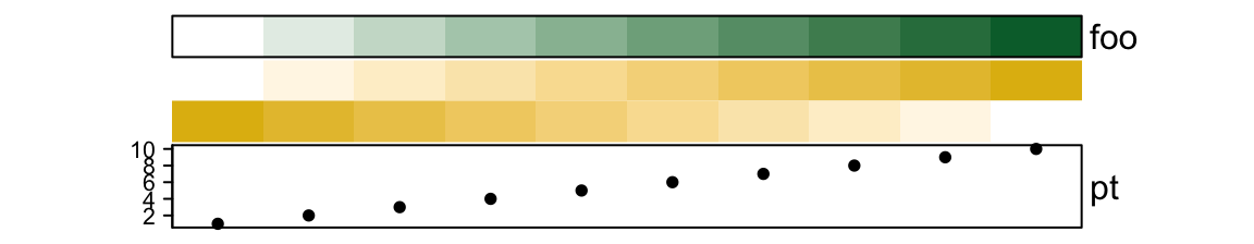
For most annotation functions implemented in ComplexHeatmap, they only draw one same type of annotation graphics, e.g. anno_points() only draws points or anno_image() only draws images. From ComplexHeatmap version 2.9.4, we added a new annotation function anno_customize(), with which you can completely freely define graphics for every annotation cell.

The input for anno_customize() should be a categorical vector.

x = c("a", "a", "a", "b", "b", "b", "c", "c", "d", "d")

For each level, you need to define a graphics function for it.

graphics = list(
    "a" = function(x, y, w, h) {
        grid.rect(x, y, w*0.8, h*0.33, gp = gpar(fill = "red"))
    },
    "b" = function(x, y, w, h) {
        grid.text("A", x, y, gp = gpar(col = "darkgreen"))
    },
    "c" = function(x, y, w, h) {
        grid.points(x, y, gp = gpar(col = "orange"), pch = 16)
    },
    "d" = function(x, y, w, h) {
        img = png::readPNG(system.file("extdata", "Rlogo.png", package = "circlize"))
        grid.raster(img, x, y, width = unit(0.8, "snpc"), 
            height = unit(0.8, "snpc")*nrow(img)/ncol(img))
    }
)

When adding graphics, each annotation cell is an independent viewport, thus, the self-defined graphics function accepts four arguments: x and y: the center of the viewport of the annotation cell, w and h: the width and height of the viewport. In the example above, we set a horizontal bar for "a", a text for "b", a point for "c" and an image for "d".

Then we add this new annotation to both row and column of the heatmap, just in the same way as normal annotations.

m = matrix(rnorm(100), 10)
Heatmap(m, 
    top_annotation = HeatmapAnnotation(foo = anno_customize(x, graphics = graphics)),
    right_annotation = rowAnnotation(bar = anno_customize(x, graphics = graphics)))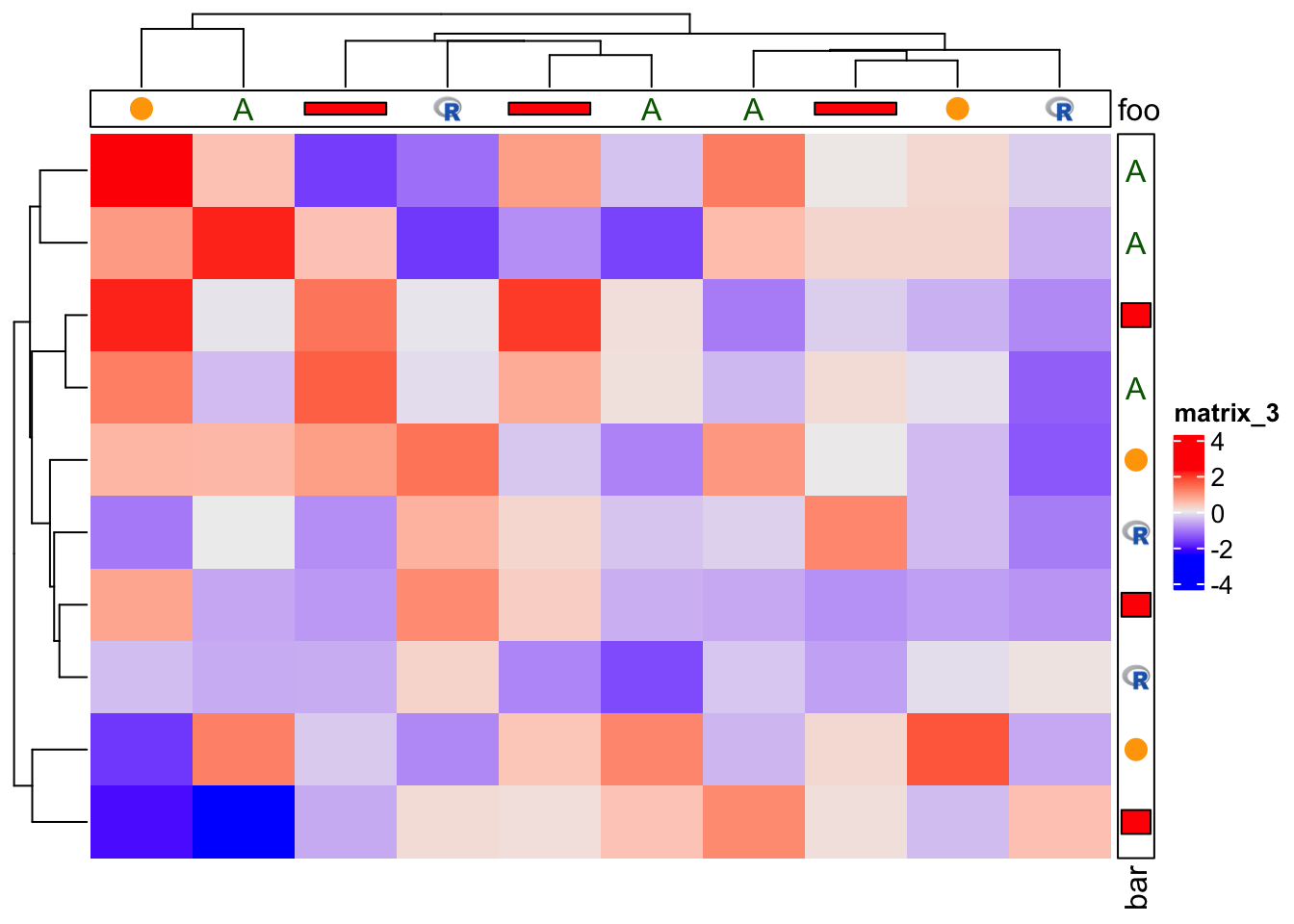

Reordering and splitting are automatically adjusted.

Heatmap(m, 
    top_annotation = HeatmapAnnotation(foo = anno_customize(x, graphics = graphics)),
    right_annotation = rowAnnotation(bar = anno_customize(x, graphics = graphics)),
    column_split = x, row_split = x)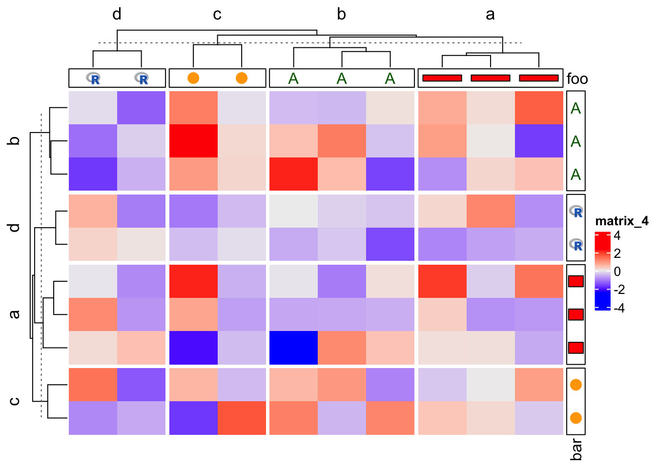

Legend() function also accepts a graphics argument, so it is easy to add legends for the “customized annotations.” How to use Legend() function will be introduced in Chapter 5.

m = matrix(rnorm(100), 10)
ht = Heatmap(m, 
    top_annotation = HeatmapAnnotation(foo = anno_customize(x, graphics = graphics)))
lgd = Legend(title = "foo", at = names(graphics), graphics = graphics)
draw(ht, annotation_legend_list = lgd)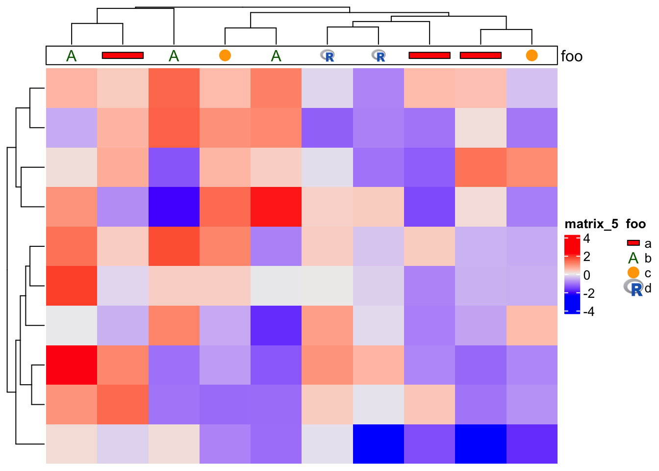

3.17 Mark annotation

Sometimes there are many rows or columns in the heatmap and we want to mark some of them. anno_mark() is used to mark subset of rows or columns and connect to labels with lines.

anno_mark() at least needs two arguments where at are the indices to the original matrix and labels are the corresponding text.

m = matrix(rnorm(1000), nrow = 100)
rownames(m) = 1:100
ha = rowAnnotation(foo = anno_mark(at = c(1:4, 20, 60, 97:100), 
    labels = month.name[1:10]))
Heatmap(m, name = "mat", cluster_rows = FALSE, right_annotation = ha,
    row_names_side = "left", row_names_gp = gpar(fontsize = 4))
Heatmap(m, name = "mat", cluster_rows = FALSE, right_annotation = ha,
    row_names_side = "left", row_names_gp = gpar(fontsize = 4), row_km = 4)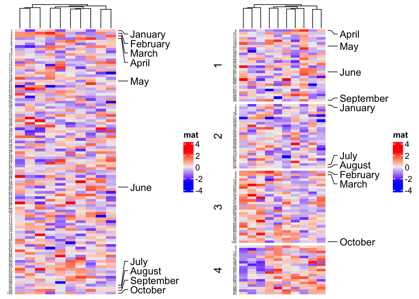

The calculation of positions of texts depends on the absolute size of the graphics device. If you resize the current interactive device or you use grid.grabExpr() to capture the current plot, you might see the positions of texts are all corrupt. Please refer to Section 10.2 for a solution.

3.18 Zoom/link annotation

anno_mark() connects single row or column on the heatmap to a label, the next annotation function anno_link() connects subsets of rows or columns to plotting regions where more comprehensive graphics can be added there. See following example where we make boxplot for every row group.

set.seed(123)
m = matrix(rnorm(100*10), nrow = 100)
subgroup = sample(letters[1:3], 100, replace = TRUE, prob = c(1, 5, 10))
rg = range(m)
panel_fun = function(index, nm) {
    pushViewport(viewport(xscale = rg, yscale = c(0, 2)))
    grid.rect()
    grid.xaxis(gp = gpar(fontsize = 8))
    grid.boxplot(m[index, ], pos = 1, direction = "horizontal")
    popViewport()
}
anno = anno_link(align_to = subgroup, which = "row", panel_fun = panel_fun, 
    size = unit(2, "cm"), gap = unit(1, "cm"), width = unit(4, "cm"))
Heatmap(m, name = "mat", right_annotation = rowAnnotation(foo = anno), 
    row_split = subgroup)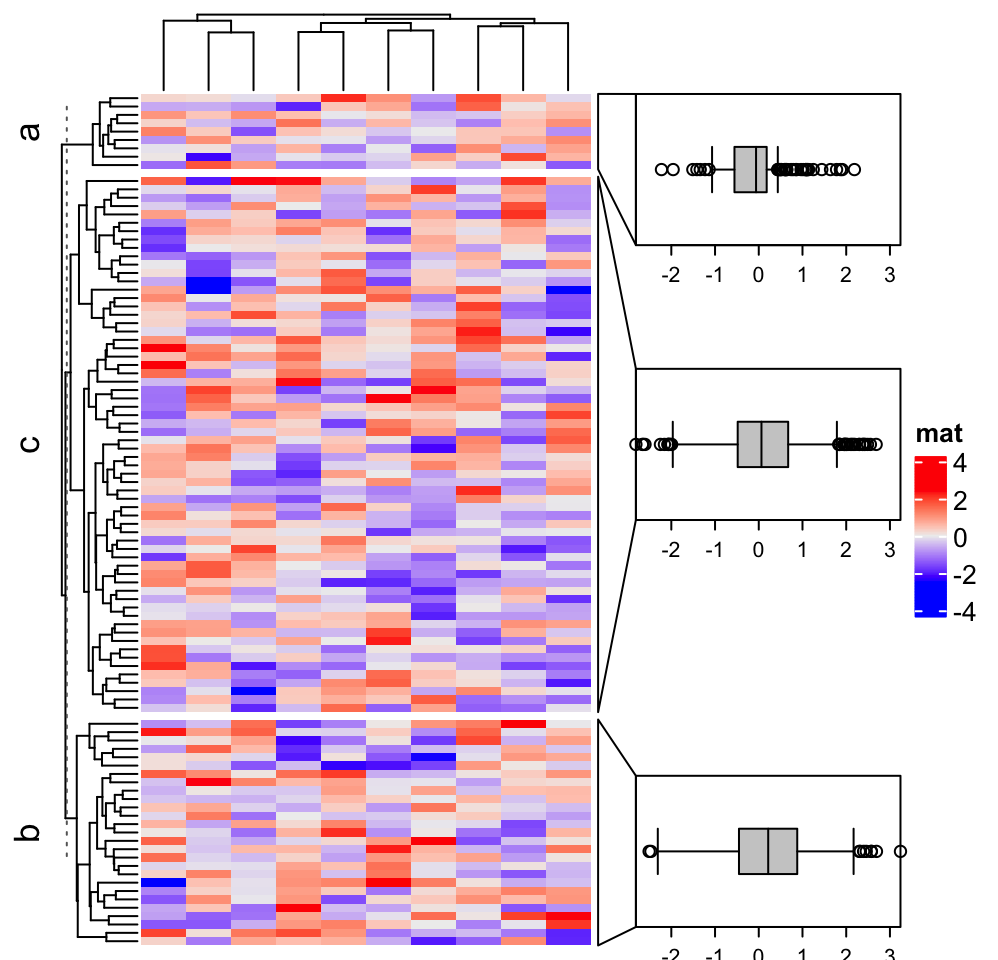

The important arguments for anno_zoom() are:

1. align_to: It defines how the plotting regions (or the boxes) correspond to the rows or the columns in the heatmap. If the value is a list of indices, each box corresponds to the rows or columns with indices in one vector in the list. If the value is a categorical variable (e.g. a factor or a character vector) that has the same length as the rows or columns in the heatmap, each box corresponds to the rows/columns in each level in the categorical variable.
2. panel_fun: A self-defined function that defines how to draw graphics in the box. The function must have a index argument which is the indices for the rows/columns that the box corresponds to. It can have a second argument nm which is the “name” of the selected part in the heatmap. The corresponding value for nm comes from align_to if it is specified as a categorical variable or a list with names.
3. size: The size of boxes. It can be pure numeric that they are treated as relative fractions of the total height/width of the heatmap. The value of size can also be absolute units.
4. gap: Gaps between boxes. It should be a unit object.

In previous example, align_to is set as a categorical variable. In the next example, align_to is set as a list of indicies and only cover slices “a” and “b.”

align_to = split(1:nrow(m), subgroup)
align_to = align_to[c("a", "b")]
anno = anno_link(align_to = align_to, which = "row", panel_fun = panel_fun, 
    size = unit(2, "cm"), gap = unit(1, "cm"), width = unit(4, "cm"))
Heatmap(m, name = "mat", right_annotation = rowAnnotation(foo = anno), 
    row_split = subgroup)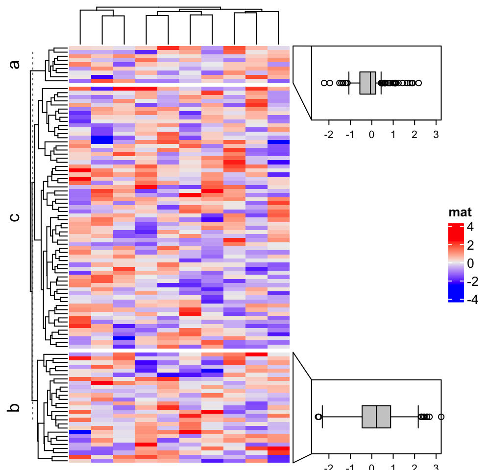

anno_link() also works for column annotations.

Similar as anno_mark(), the positions of the plotting regions also depends on the absolute size of the graphic device. If you resize the current interactive device or you use grid.grabExpr() to capture the current plot, you might see the positions of texts are all corrupt. Please refer to Section 10.2 for a solution.

As show in the previous examples, anno_link() normally works together with row_split/column_split to associate additional graphics to slices. However, it is not necessary, as long as rows with indices in align_to are continuously adjacent on heatmaps.

align_to = list(1:20)
anno = anno_link(align_to = align_to, which = "row", panel_fun = panel_fun, 
    size = unit(2, "cm"), gap = unit(1, "cm"), width = unit(4, "cm"))
# here row indices 1 to 20 are adjacent since no clustering is applied on rows
Heatmap(m, name = "mat", right_annotation = rowAnnotation(foo = anno), 
    cluster_rows = FALSE)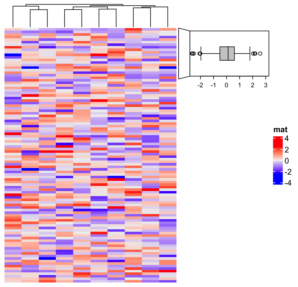

3.19 Text box annotation

From ComplexHeatmap 2.11.1, there are supports for drawing text boxes and associating them to heatmaps.

3.19.1 Construct the text box

Text box annotation depends on the text box “grob.” The text box grob can be constructed with the function textbox_grob(). It accpets a character vector with words or phrases/sentences. We first demonstrate the use of words.

Following functionn random_text() generates a vector of random words or phrases.

random_text = function(n, n_words = 1) {
    sapply(1:n, function(i) {
         w = replicate(sample(n_words, 1), 
            paste0(sample(letters, sample(4:10, 1)), collapse = ""))
        if(n_words > 1) {
            paste(w, collapse = " ")
        } else {
            w
        }
    })
}

Following code shows how to set graphics parameters:

set.seed(123)
words = random_text(10)
words

##  [1] "sncjrkeyti" "hgjisd"     "kgul"       "mgixj"      "ugzfbe"    
##  [6] "mrafuoi"    "ptfkh"      "gpqvrxbdm"  "sytvnchpl"  "nczg"

grid.newpage()
gb = textbox_grob(words)
grid.draw(gb)

grid.newpage()
gb = textbox_grob(words, gp = gpar(col = 1:10))
grid.draw(gb)

grid.newpage()
gb = textbox_grob(words, gp = gpar(fontsize = runif(10, 5, 20)))
grid.draw(gb)

Following code shows how to set the background:

grid.newpage()
gb = textbox_grob(words, background_gp = gpar(fill = "#CCCCCC", col = "#808080"))
grid.draw(gb)

grid.newpage()
gb = textbox_grob(words, background_gp = gpar(fill = "#CCCCCC", col = NA), 
    round_corners = TRUE)
grid.draw(gb)

grid.newpage()
gb = textbox_grob(words, background_gp = gpar(fill = "#CCCCCC", col = "#808080"), 
    padding = unit(4, "mm"))
grid.draw(gb)

Following code shows how to set spaces between words and lines, and how to set the width of the text box:

grid.newpage()
gb = textbox_grob(words, line_space = unit(5, "mm"))
grid.draw(gb)

grid.newpage()
gb = textbox_grob(words, text_space = unit(5, "mm"))
grid.draw(gb)

grid.newpage()
gb = textbox_grob(words, max_width = unit(12, "cm"))
grid.draw(gb)

Words can be added from the bottom left of the box or from the top left:

fontsize = sort(runif(10, 5, 20))
grid.newpage()
gb = textbox_grob(words, gp = gpar(fontsize = fontsize))
grid.draw(gb)

grid.newpage()
gb = textbox_grob(words, gp = gpar(fontsize = fontsize), 
    first_text_from = "bottom")
grid.draw(gb)

Sentences or phrases are composed of several words, so there are some extra parameters. If the longest sentence is longer than max_width, the width of the longest sentence will be the width of the text box. Setting word_wrap = TRUE can adjust the text according to the width of the text box.

sentences = random_text(5, 8)
sentences

## [1] "ihztacybvx gmtnpzdyls"                               
## [2] "ilhgo qkgscf djqphuclne fiatnsebx"                   
## [3] "dkevzsc gewi xque bvrdjoh"                           
## [4] "ekoxjw"                                              
## [5] "lidcgxh exfdckjz kjos jmxcrzh jgyfqta jmzbovhc fnosi"

fontsize = runif(5, 5, 20)
grid.newpage()
gb = textbox_grob(sentences, gp = gpar(col = 1:5, fontsize = fontsize))
grid.draw(gb)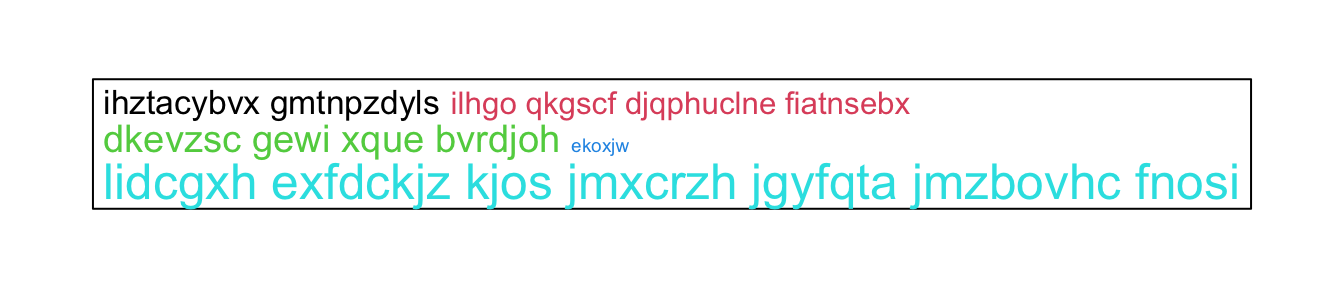

grid.newpage()
gb = textbox_grob(sentences, gp = gpar(col = 1:5, fontsize = fontsize), 
    word_wrap = TRUE)
grid.draw(gb)

Also argument add_new_line can be set to TRUE so each sentence will be in a single line.

grid.newpage()
gb = textbox_grob(sentences, gp = gpar(col = 1:5, fontsize = fontsize), 
    add_new_line = TRUE)
grid.draw(gb)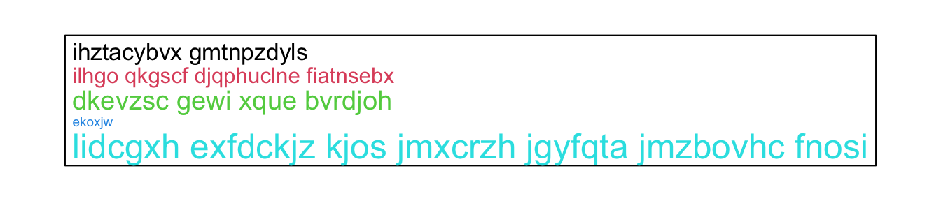

grid.newpage()
gb = textbox_grob(sentences, gp = gpar(col = 1:5, fontsize = fontsize), 
    add_new_line = TRUE, word_wrap = TRUE)
grid.draw(gb)

Finally, the width and height of the text box grob can be obtained by grobWidth() and grobHeight(). Also there is a companion function grid.textbox() that directly draws text box at a certain position.

# code only for demonstration
gb = textbox_grob(words)
grobWidth(gb)
grobHeight(gb)
grid.textbox(words, x, y)

3.19.2 Draw textbox annotation

The function anno_textbox() draws several text boxes and associate them to heatmaps. Note you don’t need to directly use textbox_grob() function with anno_textbox(), but there are parameters that control texts in anno_textbox() that are directly passed to textbox_grob().

Since texts are already wrapped into boxes, the text box annotations are basically implemented by anno_link() and anno_block().

By default, the text box annotation is implemented by anno_link(). Since heights of text boxes are not always the same as the height of subsets of rows they correspond to, there are connections between the heatmap and text boxes. In the following example, we generated 10 text boxes and each one is linked to a heatmap slice. In this case, the first parameter for anno_textbox() is a categorical variable which also split heatmap rows. The second parameter text is a named list of character vectors where name of the list should correspond to the levels in split.

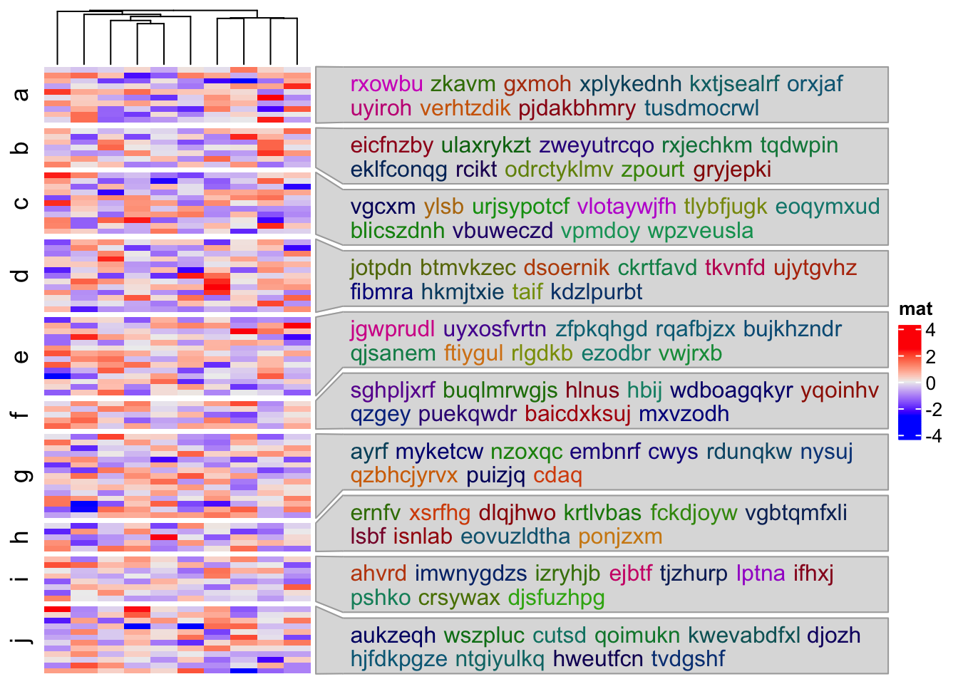
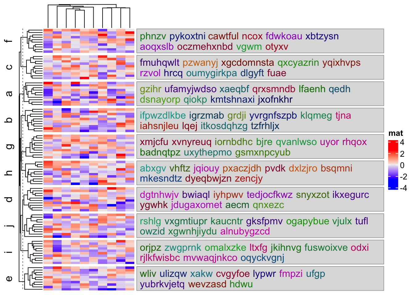
mat = matrix(rnorm(100*10), nrow = 100)
split = sample(letters[1:10], 100, replace = TRUE)
text = lapply(unique(split), function(x) {
    random_text(10)
})
names(text) = unique(split)

Heatmap(mat, name = "mat", cluster_rows = FALSE, row_split = split,
    right_annotation = rowAnnotation(textbox = anno_textbox(split, text))
)

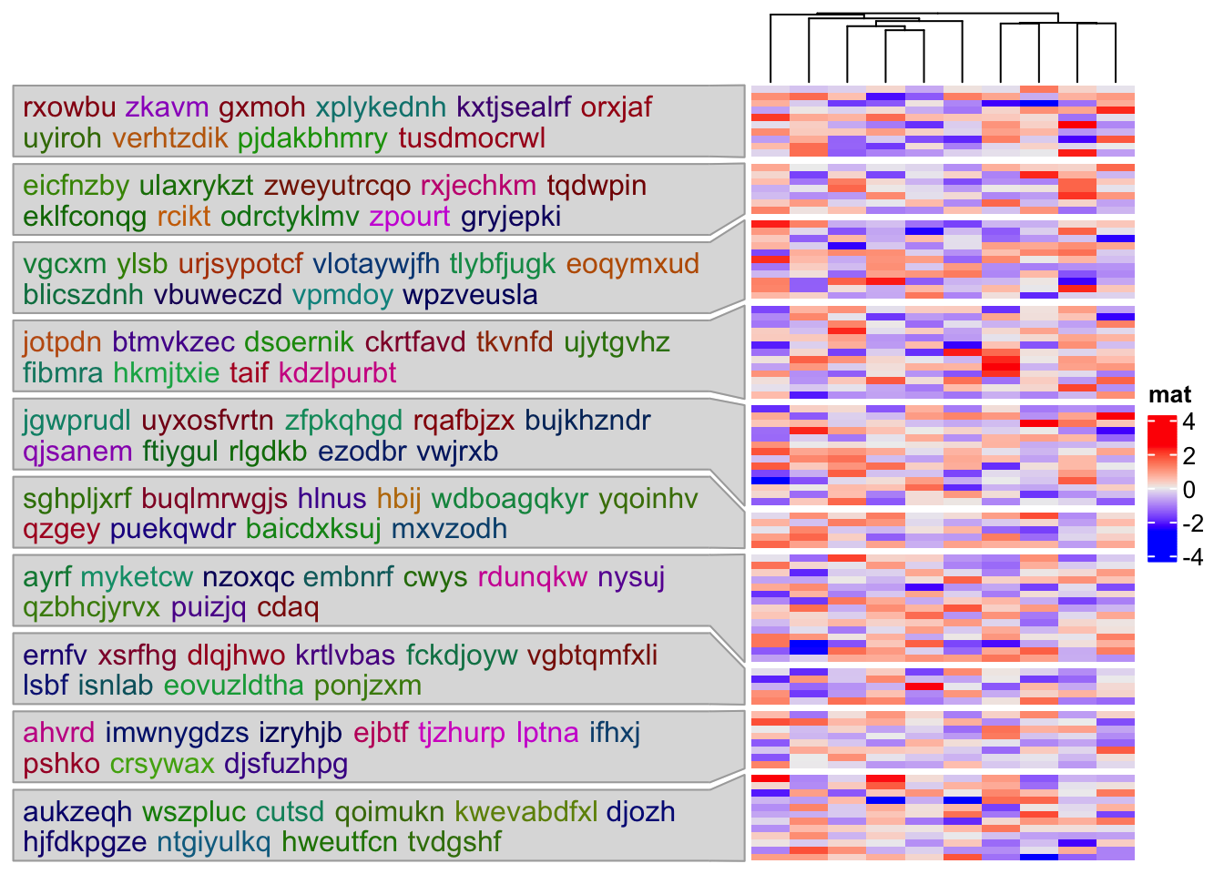
Or put on the left side of the heatmap:

Heatmap(mat, name = "mat", cluster_rows = FALSE, row_split = split, row_title = NULL,
    left_annotation = rowAnnotation(textbox = anno_textbox(split, text, side = "left"))
)

Parameters for textbox_grob() can be directly passed in anno_textbox(). E.g. when the text are sentences, to control word wrap and new lines:

split = sample(letters[1:5], 100, replace = TRUE)
sentences = lapply(unique(split), function(x) {
    random_text(3, 8)
})
names(sentences) = unique(split)

Heatmap(mat, name = "mat", row_split = split,
    right_annotation = rowAnnotation(
        textbox = anno_textbox(
            split, sentences, 
            word_wrap = TRUE, 
            add_new_line = TRUE)
    )
)

The first argument for anno_textbox() can also be set as a list of indicies. Note the indices for rows should be continuously adjacent on heatmaps.

align_to = split(seq_along(split), split)
Heatmap(mat, name = "mat", row_split = split,
    right_annotation = rowAnnotation(
        textbox = anno_textbox(
            align_to[c("a", "b")], 
            sentences[c("a", "b")], # names should match
            word_wrap = TRUE, 
            add_new_line = TRUE)
    )
)

anno_textbox() works mainly together with row_split to associate more information to every heatmap slice. But this is not necessary, as long as you can ensure the indices are continuously adjacent on heatmaps. In the next example, rows are not clustered, we add two text boxed to correspond to row 1-10 and row 11-30.

Heatmap(mat, name = "mat", cluster_rows = FALSE,
    right_annotation = rowAnnotation(
        textbox = anno_textbox(
            list("a" = 1:10, "b" = 11:30), 
            sentences[c("a", "b")], 
            word_wrap = TRUE, 
            add_new_line = TRUE)
    )
)

There are some cases that users want to put the text boxes exactly at the positions of the corresponding heatmap slices. In this case, the by argument should be set to "anno_block". And now anno_block() is internally used to implement text box annotations.

split = rep(letters[1:10], 10)
text = lapply(unique(split), function(x) {
    random_text(10)
})
names(text) = unique(split)

Heatmap(mat, name = "mat", row_split = split,
    right_annotation = rowAnnotation(
        textbox = anno_textbox(split, text, by = "anno_block")
    )
)

Similarly, the first parameter can be set as a list of indicies:

align_to = split(seq_along(split), split)
Heatmap(mat, name = "mat", row_split = split,
    right_annotation = rowAnnotation(
        textbox = anno_textbox(
            align_to[c("a", "b")], 
            text[c("a", "b")], # names should match
            by = "anno_block")
    )
)

Heatmap(mat, name = "mat", cluster_rows = FALSE,
    right_annotation = rowAnnotation(
        textbox = anno_textbox(
            list("a" = 1:10, "b" = 50:70), 
            text[c("a", "b")], 
            by = "anno_block"))
)

So far, the texts are assigned with random colors. Now the question is how to exactly control graphics parameters for texts in the text boxes. In previous examples, the value of text is a list of character vectors. The graphics parameters can be integrated into text by setting text as a list of data frames. In each data frame, the first column contains texts that will be put into boxes. The data frame can also contains the following four columns ("col", "fontsize", "fontfamily" and "fontface") to exactly control the corresponding text.

split = rep(letters[1:5], 20)
text = lapply(unique(split), function(x) {
    df = data.frame(text = random_text(10))
    df$fontsize = runif(10, 6, 20)
    if(runif(1) > 0.5) {
        df$col = rep(rand_color(1), 10)
    } else {
        df$col = 1:10
    }
    df
})
names(text) = unique(split)
head(text[[1]])

##         text  fontsize       col
## 1 gixsnwmyjr 16.409436 #E80DF8FF
## 2    klxdszq 14.065497 #E80DF8FF
## 3    nmyaiko 10.148988 #E80DF8FF
## 4  iytaznevh  9.719641 #E80DF8FF
## 5  wbqlhxiof 19.864118 #E80DF8FF
## 6   zaovsbwe 14.295501 #E80DF8FF

Heatmap(mat, name = "mat", cluster_rows = FALSE, row_split = split,
    right_annotation = rowAnnotation(textbox = anno_textbox(split, text))
)

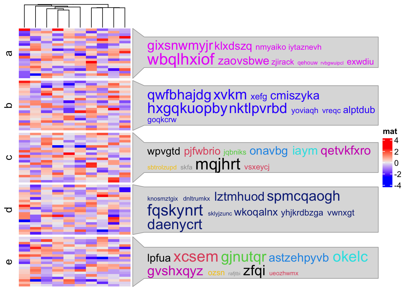
In the simplifyEnrichment package, we use anno_textbox() to implement a word cloud annotation to visualize summaries of biological functions in each GO cluster.

3.20 Summary annotation

There is one special annotation anno_summary() which only works with one-column heatmap or one-row heatmap (we can say the heatmap only contains a vector). It shows summary statistics for the vector in the heatmap. If the corresponding vector is discrete, the summary annotation is presented as barplots and if the vector is continuous, the summary annotation is boxplot. anno_summary() is always used when the heatmap is split so that statistics can be compared between heatmap slices.

The first example shows the summary annotation for discrete heatmap. The barplot shows the proportion of each level in each slice. The absolute values can already be seen by the height of the heatmap slice.

The color schema for the barplots is automatically extracted from the heatmap.

ha = HeatmapAnnotation(summary = anno_summary(height = unit(4, "cm")))
v = sample(letters[1:2], 50, replace = TRUE)
split = sample(letters[1:2], 50, replace = TRUE)

Heatmap(v, name = "mat", col = c("a" = "red", "b" = "blue"),
    top_annotation = ha, width = unit(2, "cm"), row_split = split)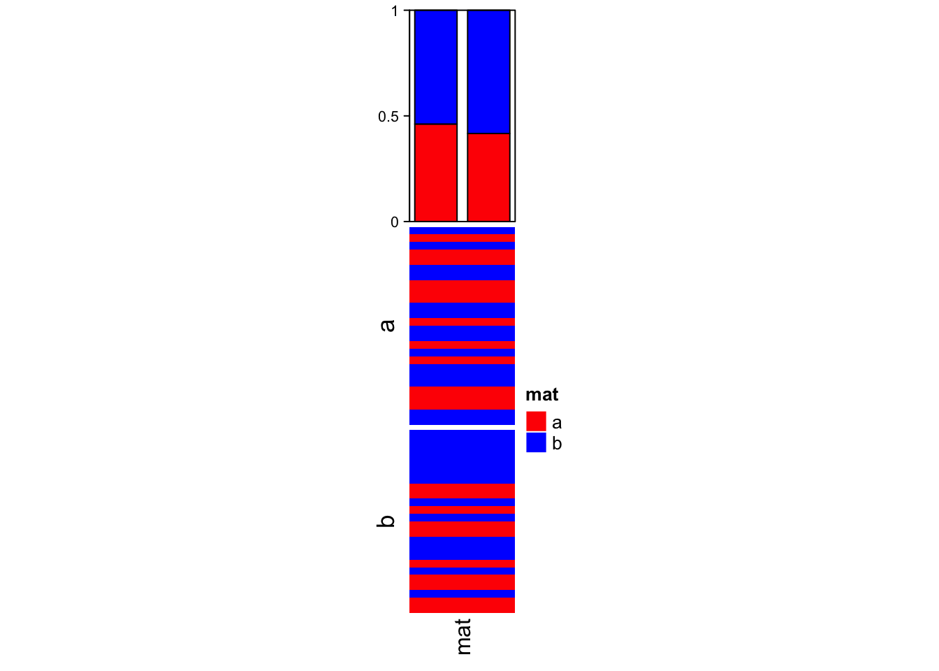

The second example shows the summary annotation for continuous heatmap. The graphic parameters should be manually set by gp. The legend of the boxplot can be created and added as introduced in Section 5.2, last second paragraph.

ha = HeatmapAnnotation(summary = anno_summary(gp = gpar(fill = 2:3), 
    height = unit(4, "cm")))
v = rnorm(50)
Heatmap(v, name = "mat", top_annotation = ha, width = unit(2, "cm"), 
    row_split = split)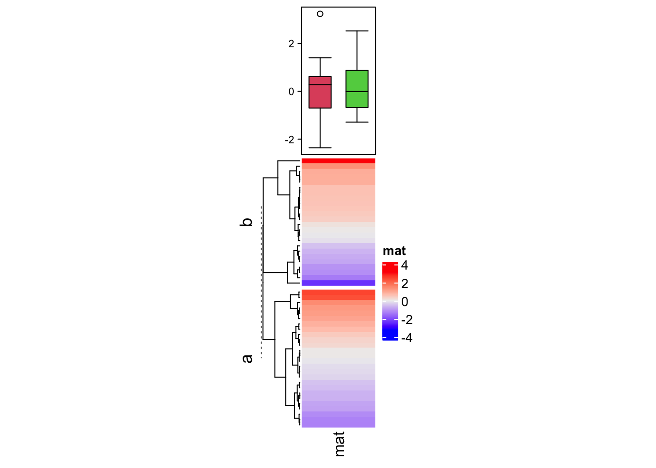

Normally we don’t draw this one-column heatmap along. It is always combined with other “main heatmaps.” E.g. A gene expression matrix with a one-column heatmap which shows whether the gene is a protein coding gene or a linc-RNA gene.

In following, we show a simple example of a “main heatmap” with two one-column heatmaps. The functionality of heatmap concatenation will be introduced in Chapter 4.

m = matrix(rnorm(50*10), nrow = 50)
ht_list = Heatmap(m, name = "main_matrix")

ha = HeatmapAnnotation(summary = anno_summary(height = unit(3, "cm")))
v = sample(letters[1:2], 50, replace = TRUE)
ht_list = ht_list + Heatmap(v, name = "mat1", top_annotation = ha, width = unit(1, "cm"))

ha = HeatmapAnnotation(summary = anno_summary(gp = gpar(fill = 2:3), 
    height = unit(3, "cm")))
v = rnorm(50)
ht_list = ht_list + Heatmap(v, name = "mat2", top_annotation = ha, width = unit(1, "cm"))

split = sample(letters[1:2], 50, replace = TRUE)
lgd_boxplot = Legend(labels = c("group a", "group b"), title = "group",
    legend_gp = gpar(fill = c("red", "blue")))
draw(ht_list, row_split = split, ht_gap = unit(5, "mm"), 
    heatmap_legend_list = list(lgd_boxplot))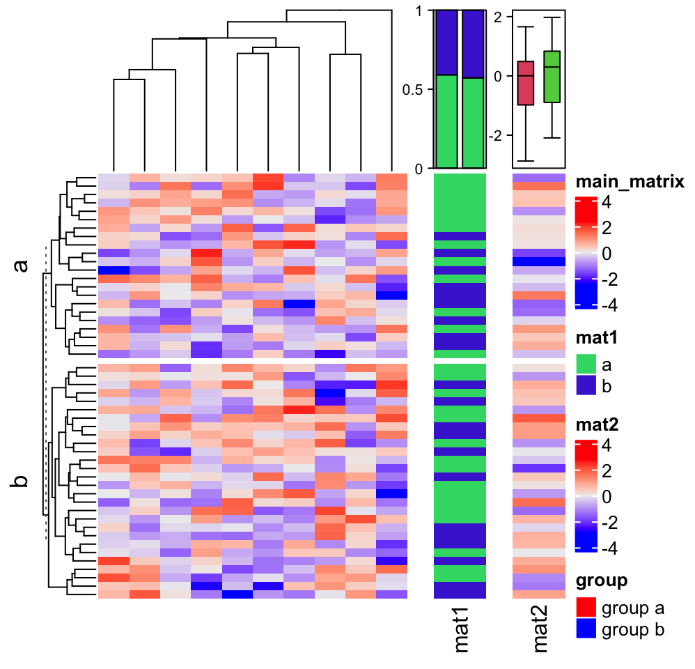

3.21 Multiple annotations

3.21.1 General settings

As mentioned before, to put multiple annotations in HeatmapAnnotation(), they just need to be specified as name-value pairs. In HeatmapAnnotation(), there are some arguments which controls multiple annotations. For these arguments, they are specified as a vector which has same length as number of the annotations, or a named vector with subset of the annotations.

The simple annotations which are specified as vectors, matrices and data frames will automatically have legends on the heatmap. show_legend controls whether to draw the legends for them. Note here if show_legend is a vector, the value of show_legend should be in one of the following formats:

• A logical vector with the same length as the number of simple annotations.
• A logical vector with the same length as the number of totla annotations. The values for complex annotations are ignored.
• A named vector to control subset of the simple annotations.

For customization on the annotation legends, please refer to Section 5.4.

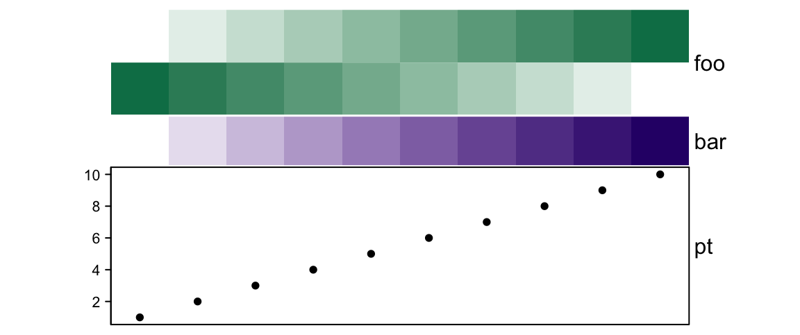
ha = HeatmapAnnotation(foo = 1:10, 
    bar = cbind(1:10, 10:1),
    pt = anno_points(1:10),
    show_legend = c("bar" = FALSE)
)
Heatmap(matrix(rnorm(100), 10), name = "mat", top_annotation = ha)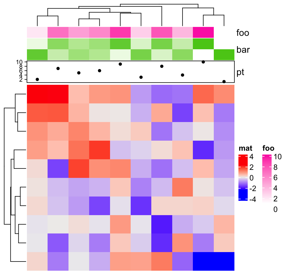

gp controls graphic parameters (except fill) for the simple annotatios, such as the border of annotation grids.

ha = HeatmapAnnotation(foo = 1:10, 
    bar = cbind(1:10, 10:1),
    pt = anno_points(1:10),
    gp = gpar(col = "red")
)

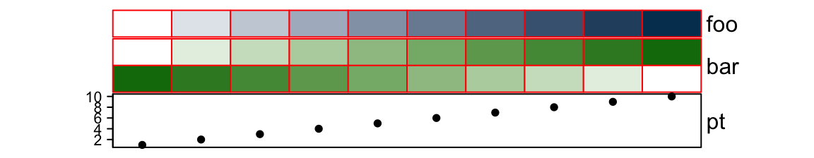
border controls the border of every single annotations. show_annotation_name controls whether show annotation names. As mentioned, the value can be a single value, a vector or a named vector.

ha = HeatmapAnnotation(foo = 1:10, 
    bar = cbind(1:10, 10:1),
    pt = anno_points(1:10),
    show_annotation_name = c(bar = FALSE), # only turn off `bar`
    border = c(foo = TRUE) # turn on foo
)

annotation_name_gp, annotation_name_offset, annotation_name_side and annotation_name_rot control the style and position of the annotation names. The latter three can be specified as named vectors. If annotation_name_offset is specified as a named vector, it can be specified as characters while not unit objects: annotation_name_offset = c(foo = "1cm").

gap controls the space between every two neighbouring annotations. The value can be a single unit or a vector of units.

ha = HeatmapAnnotation(foo = 1:10, 
    bar = cbind(1:10, 10:1),
    pt = anno_points(1:10),
    gap = unit(2, "mm"))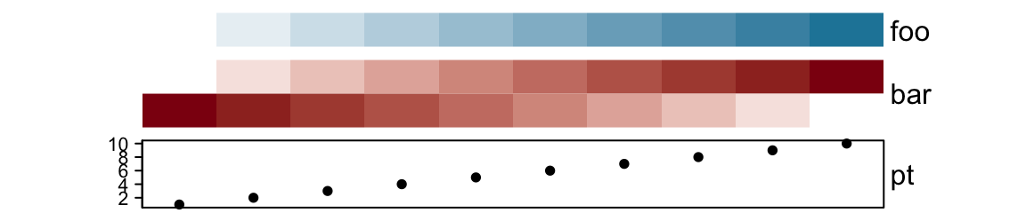

ha = HeatmapAnnotation(foo = 1:10, 
    bar = cbind(1:10, 10:1),
    pt = anno_points(1:10),
    gap = unit(c(2, 10), "mm"))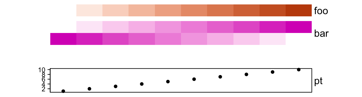

3.21.2 Size of annotations

height, width, annotation_height and annotation_width control the height or width of the complete heatmap annotations. Normally you don’t need to set them because all the single annotations have fixed height/width and the final height/width for the whole heatmap annotation is the sum of them. Resizing these values will involve rather complicated adjustment depending on whether it is a simple annotation or complex annotation. The resizing of heatmap annotations will also happen when adjusting a list of heatmaps. In following examples, we take column annotations as examples and demonstrate some scenarios for the resizing adjustment.

First the default height of ha:

# foo: 1cm, bar: 5mm, pt: 1cm
ha = HeatmapAnnotation(foo = cbind(1:10, 10:1), 
    bar = 1:10,
    pt = anno_points(1:10))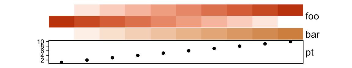

If height is set, the size of the simple annotation will not change, while only the complex annotations are adjusted. If there are multiple complex annotations, they are adjusted according to the ratio of their original size.

# foo: 1cm, bar: 5mm, pt: 4.5cm
ha = HeatmapAnnotation(foo = cbind(1:10, 10:1), 
    bar = 1:10,
    pt = anno_points(1:10),
    height = unit(6, "cm"))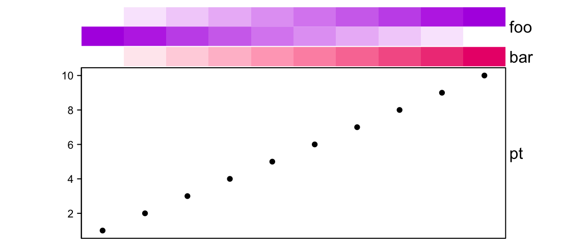

simple_anno_size controls the height of all simple annotations. Recall ht_opt$simple_anno_size can be set to globally control the size of simple annotations in all heatmaps.

# foo: 2cm, bar:1cm, pt: 3cm
ha = HeatmapAnnotation(foo = cbind(1:10, 10:1), 
    bar = 1:10,
    pt = anno_points(1:10),
    simple_anno_size = unit(1, "cm"), height = unit(6, "cm"))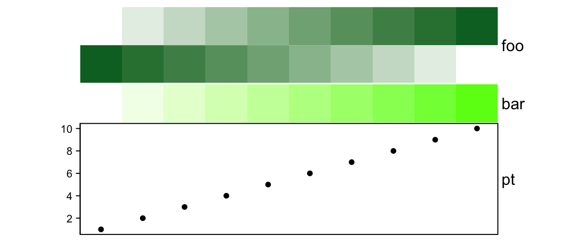

If annotation_height is set as a vector of absolute units, the height of all three annotations are adjusted accordingly.

# foo: 1cm, bar: 2cm, pt: 3cm
ha = HeatmapAnnotation(foo = cbind(1:10, 10:1), 
    bar = 1:10,
    pt = anno_points(1:10),
    annotation_height = unit(1:3, "cm"))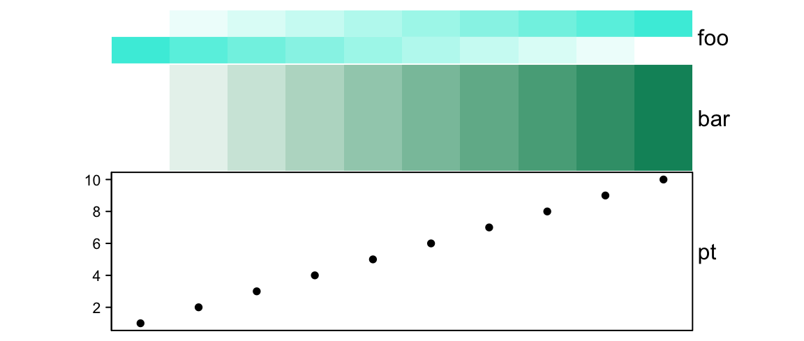

If annotation_height is set as pure numbers which is treated as relative ratios for annotations, height should also be set as an absolute unit and the size of every single annotation is adjusted by the ratios.

# foo: 1cm, bar: 2cm, pt: 3cm
ha = HeatmapAnnotation(foo = cbind(1:10, 10:1), 
    bar = 1:10,
    pt = anno_points(1:10),
    annotation_height = 1:3, height = unit(6, "cm"))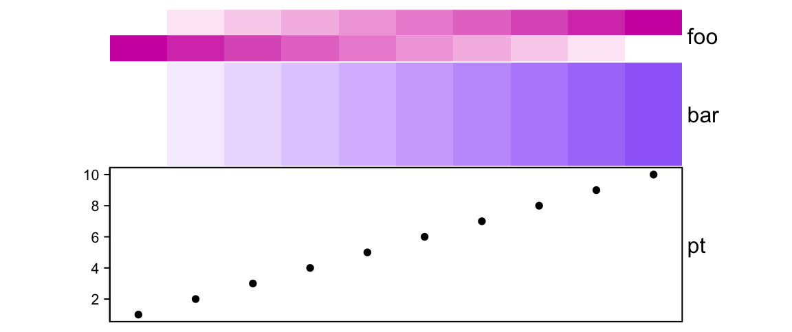

annotation_height can be mixed with relative units (in null unit) and absolute units.

# foo: 1.5cm, bar: 1.5cm, pt: 3cm
ha = HeatmapAnnotation(foo = cbind(1:10, 10:1), 
    bar = 1:10,
    pt = anno_points(1:10),
    annotation_height = unit(c(1, 1, 3), c("null", "null", "cm")), height = unit(6, "cm")
)

# foo: 2cm, bar: 1cm, pt: 3cm
ha = HeatmapAnnotation(foo = cbind(1:10, 10:1), 
    bar = 1:10,
    pt = anno_points(1:10),
    annotation_height = unit(c(2, 1, 3), c("cm", "null", "cm")), height = unit(6, "cm")
)

If there are only simple annotations, simply setting height won’t change the height.

# foo: 1cm, bar: 5mm
ha = HeatmapAnnotation(foo = cbind(1:10, 10:1), 
    bar = 1:10,
    height = unit(6, "cm"))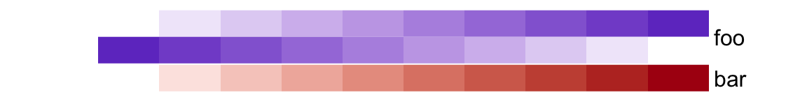

unless simple_anno_size_adjust is set to TRUE.

# foo: 4cm, bar: 2cm
ha = HeatmapAnnotation(foo = cbind(1:10, 10:1), 
    bar = 1:10,
    height = unit(6, "cm"),
    simple_anno_size_adjust = TRUE)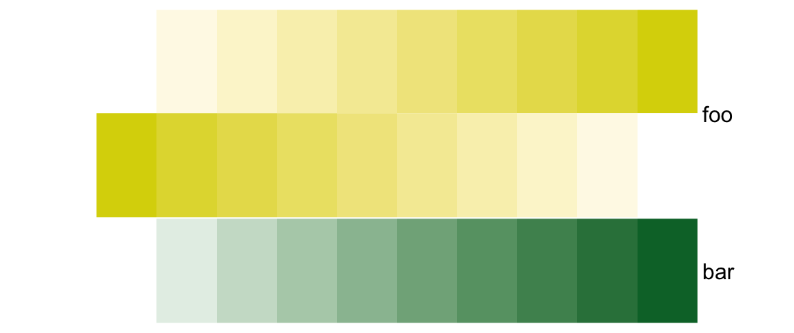

Section 4.6 introduces how the annotation sizes are adjusted among a list of heatmaps.

3.21.3 Annotation labels

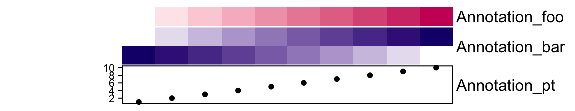
From version 2.3.3, alternative labels for annotations can be set by annotation_label argument:

ha = HeatmapAnnotation(foo = 1:10, 
    bar = cbind(1:10, 10:1),
    pt = anno_points(1:10),
    annotation_label = c("Annotation_foo", "Annotation_bar", "Annotation_pt")
)

Annotation labels can also be set with complex text:

ha = HeatmapAnnotation(foo = 1:10, 
    bar = cbind(1:10, 10:1),
    pt = anno_points(1:10),
    annotation_label = gt_render(
        c("**Anno**_<span style='color:red'>foo</span>", 
          "**Anno**_<span style='color:blue'>bar</span>", 
          "**Anno**_<span style='color:green'>pt</span>"),
        gp = gpar(box_fill = "grey")
    )
)
Heatmap(matrix(rnorm(100), 10), name = "mat", top_annotation = ha)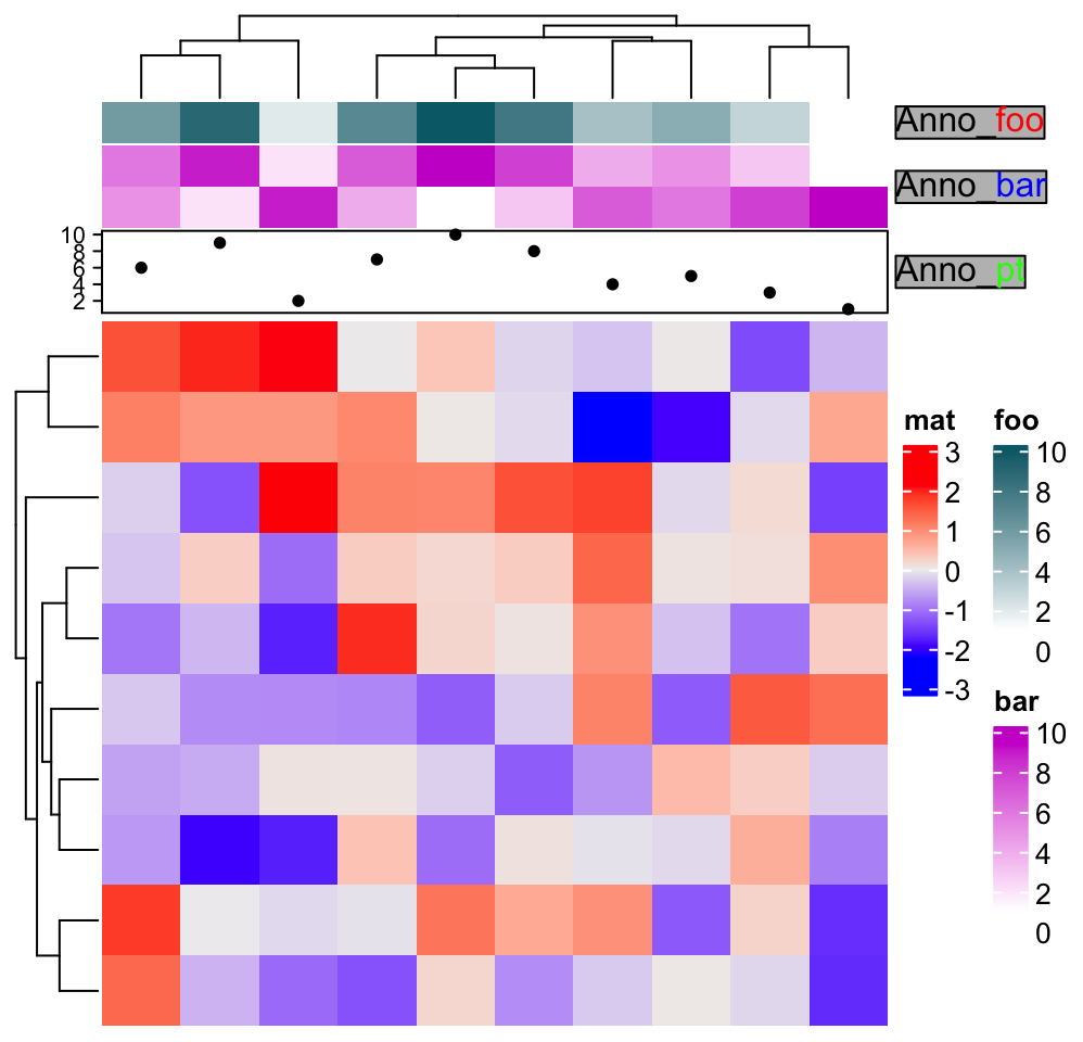

From version 2.5.6, rotations of annotation names can be configured.

ha = HeatmapAnnotation(foo = 1:10, 
    bar = cbind(1:10, 10:1),
    pt = anno_points(1:10),
    annotation_name_rot = 45
)
Heatmap(matrix(rnorm(100), 10), name = "mat", top_annotation = ha)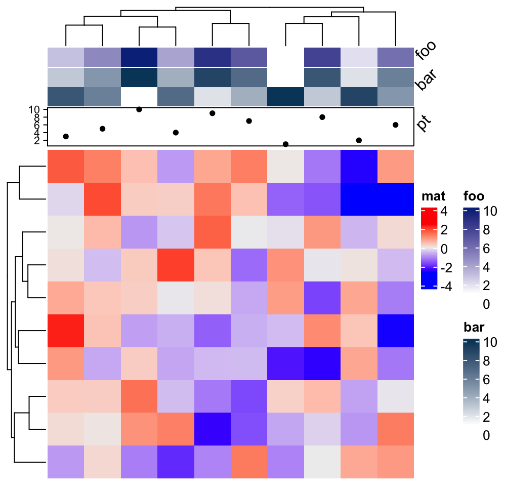

Or on the rows:

ha = rowAnnotation(foo = 1:10, 
    bar = cbind(1:10, 10:1),
    pt = anno_points(1:10),
    annotation_name_rot = 45
)
Heatmap(matrix(rnorm(100), 10), name = "mat", left_annotation = ha)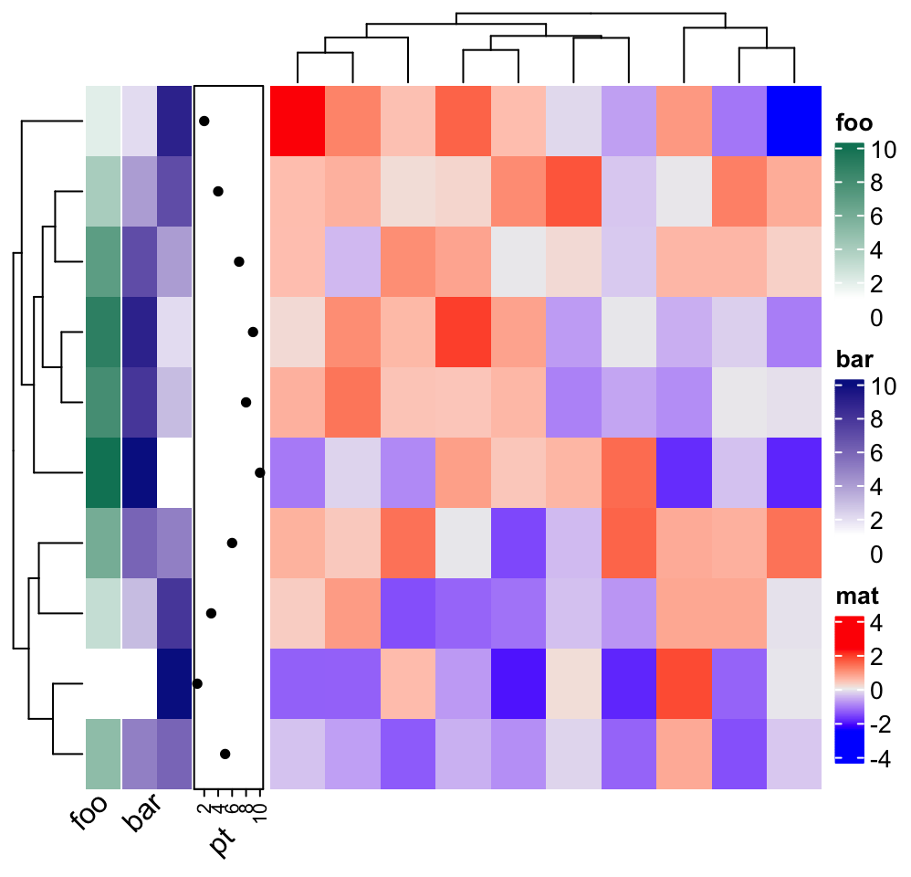

3.22 Utility functions

There are some utility functions which make the manipulation of heatmap annotation easier. Just see following examples.

ha = HeatmapAnnotation(foo = 1:10, 
    bar = cbind(1:10, 10:1),
    pt = anno_points(1:10))
length(ha)

## [1] 3

nobs(ha)

## [1] 10

Get or set the names of the annotations:

names(ha)

## [1] "foo" "bar" "pt"

names(ha) = c("FOO", "BAR", "PT")
names(ha)

## [1] "FOO" "BAR" "PT"

You can concatenate two HeatmapAnnotation objects if they contain same number of observations and different annotation names.

ha1 = HeatmapAnnotation(foo = 1:10, 
    bar = cbind(1:10, 10:1),
    pt = anno_points(1:10))
ha2 = HeatmapAnnotation(FOO = runif(10), 
    BAR = sample(c("a", "b"), 10, replace = TRUE),
    PT = anno_points(rnorm(10)))
ha = c(ha1, ha2)
names(ha)

## [1] "foo" "bar" "pt"  "FOO" "BAR" "PT"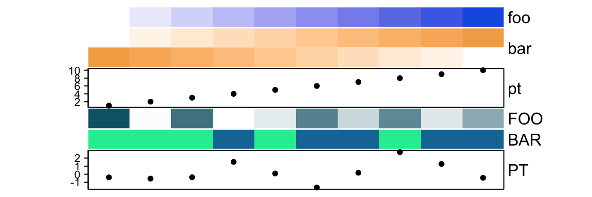

HeatmapAnnotation object sometimes is subsettable. The row index corresponds to observations in the annotation and column index corresponds to the annotations. If the annotations are all simple annotations or the complex annotation created by anno_*() functions in ComplexHeatmap package, the HeatmapAnnotation object is always subsettable.

ha_subset = ha[1:5, c("foo", "PT")]
ha_subset

## A HeatmapAnnotation object with 2 annotations
##   name: heatmap_annotation_136 
##   position: column 
##   items: 5 
##   width: 1npc 
##   height: 15.3514598035146mm 
##   this object is subsettable
##   5.21733333333333mm extension on the left 
##   6.75733333333333mm extension on the right 
## 
##  name   annotation_type color_mapping height
##   foo continuous vector        random    5mm
##    PT     anno_points()                 10mm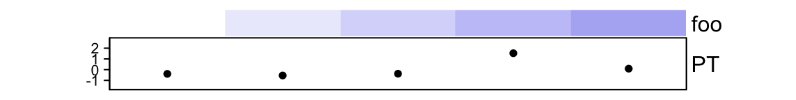

The construction of heatmaps and annotations can be separated, later the annotations can be filled into the heatmap objects by the attach_annotation() function.

# code only for demonstration
ha1 = HeatmapAnnotation(foo = 1:10)
ha2 = rowAnnotation(bar = letters[1:10])
ht = Heatmap(mat)
ht = attach_annotation(ht, ha1, side = "top")
ht = attach_annotation(ht, ha2, side = "left")

3.23 Implement new annotation functions

All the annotation functions defined in ComplexHeatmap are constructed by the AnnotationFunction class. The AnnotationFunction class not only stores the “real R function” which draws the graphics, it also calculates the spaces produced by the annotation axis. More importantly, it allows splitting the annotation graphics according to the split of the main heatmap.

As expected, the main part of the AnnotationFunction class is a function which defines how to draw at specific positions which correspond to rows or columns in the heatmap. The function should have three arguments: index, k and n (the names of the arguments can be arbitrary) where k and n are optional. index corresponds to the indices of rows or columns of the heatmap. The value of index is not necessarily to be the whole row indices or column indices in the heatmap. It can also be a subset of the indices if the annotation is split into slices according to the split of the heatmap. index is reordered according to the reordering of heatmap rows or columns (e.g. by clustering). So, index actually contains a list of row or column indices for the current slice after row or column reordering.

As mentioned, annotation can be split into slices. k corresponds to the current slice and n corresponds to the total number of slices. The annotation function draws in every slice repeatedly. The information of k and n sometimes can be useful, for example, we want to add axis in the annotation, and if it is a column annotation and axis is drawn on the very right of the annotation area, the axis is only drawn when k == n.

Since the function only allows index, k and n, the function sometimes uses several external variables which can not be defined inside the function, e.g. the data points for the annotation. These variables should be imported into the AnnotationFunction class by var_import so that the function can correctly find these variables.

One important feature for AnnotationFunction class is it can be subsettable, which is the base for splitting. To allow subsetting on the object, users need to define the rule for the imported variables if there is any. The rules are simple functions which accpet the variable and indices, and return the subset of the variable. The subset rule functions implemented in this package are subset_gp(), subset_matrix_by_row() and subset_vector(). If the subsetting rule is not provided, it is inferred by the type of the object.

In the following example, we first construct an AnnotationFunction object which needs external variable and supports subsetting. This annotation contains a list of “lolipops” (points plus vertical segments) which is drawn in a viewport. Y-axis is drawn in the first slices.

The variable x is from outside of the function, so it should be added to var_import.

x = 1:10
anno1 = AnnotationFunction(
    fun = function(index, k, n) {
        n = length(index)
        pushViewport(viewport(xscale = c(0.5, n + 0.5), yscale = c(0, 10)))
        grid.rect()
        grid.points(1:n, x[index], default.units = "native")
        grid.segments(1:n, 0, 1:n, x[index], default.units = "native")
        if(k == 1) grid.yaxis()
        popViewport()
    },
    var_import = list(x = x),
    n = 10,
    subsettable = TRUE,
    height = unit(2, "cm")
)
anno1

## An AnnotationFunction object
##   function: user-defined
##   position: column 
##   items: 10 
##   width: 1npc 
##   height: 2cm 
##   imported variable: x 
##   this object is subsettable

Then we can assign anno1 in HeatmapAnnotation() function. Since anno1 is subsettable, you can split columns of the heatmap.

m = rbind(1:10, 11:20)
Heatmap(m, top_annotation = HeatmapAnnotation(foo = anno1))
Heatmap(m, top_annotation = HeatmapAnnotation(foo = anno1), 
    column_split = rep(c("A", "B"), each = 5))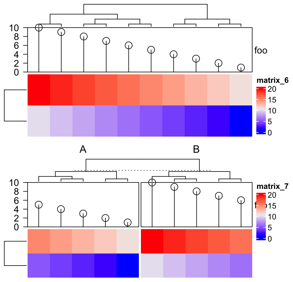

The second way is to put all data variables inside the function and no need to import other variables.

# code only for demonstration
anno2 = AnnotationFunction(
    fun = function(index) {
        x = 1:10
        n = length(index)
        pushViewport(viewport())
        grid.points(1:n, x[index])
        popViewport()
    },
    n = 10,
    subsettable = TRUE
)

The most compact way to only specify the function to the constructor. This allows reordering, but it does not work when you split heatmap.

# code only for demonstration
anno3 = AnnotationFunction(
    fun = function(index) {
        x = 1:10
        n = length(index)
        pushViewport(viewport())
        grid.points(1:n, x[index])
        popViewport()
    }
)

All the anno_*() functions introduced in this section actually are not really annotation functions, while they are functions generating annotation functions with specific configurations.

anno_points(1:10)

## An AnnotationFunction object
##   function: anno_points()
##   position: column 
##   items: 10 
##   width: 1npc 
##   height: 1cm 
##   imported variable: data_scale, axis_param, border, size, value, pch_as_image, axis, gp, axis_grob, pch 
##   subsettable variable: gp, value, size, pch 
##   this object is subsettable
##   5.13831111111111mm extension on the left

In most cases, you don’t need to manually construct your AnnotationFunction objects. The annotation function anno_*() implemented in ComplexHeatmap are already enough for most of the analysis tasks. On the other hand, users can also use anno_empty() and decorate_annotation() to quickly add self-defined annotation graphics. E.g. we can re-implement previous heatmap as (of course it is lengthy):

ht = Heatmap(m, name = "mat",
    top_annotation = HeatmapAnnotation(foo = anno_empty(height = unit(2, "cm"))), 
    column_split = rep(c("A", "B"), each = 5))
ht = draw(ht)
co = column_order(ht)
decorate_annotation("foo", slice = 1, {
    od = co[[1]]
    pushViewport(viewport(xscale = c(0.5, length(od) + 0.5), yscale = c(0, 10)))
    grid.points(seq_along(od), x[od])
    grid.segments(seq_along(od), 0, seq_along(od), x[od], default.units = "native")
    grid.yaxis()
    popViewport()
})
decorate_annotation("foo", slice = 2, {
    od = co[[2]]
    pushViewport(viewport(xscale = c(0.5, length(od) + 0.5), yscale = c(0, 10)))
    grid.points(seq_along(od), x[od])
    grid.segments(seq_along(od), 0, seq_along(od), x[od], default.units = "native")
    popViewport()
})

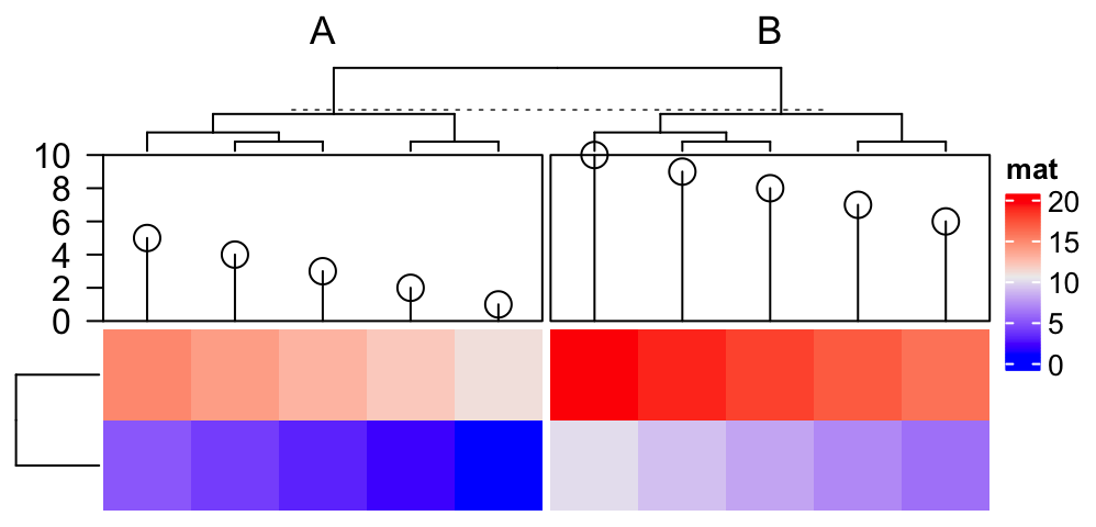
3.23.1 Construct annotation function by cell_fun

To simplify the use of AnnotationFunction(), from version 2.9.3, it has a new argument cell_fun which accepts a self-defined function that only draws in a single “annotation cell.” This would be convenient for annotation only with a few cells. See the following example which visualizes percent values by text and bars. Actually this is how anno_numeric() (Section 3.15) is implemented.

anno_pct = function(x) {

    max_x = max(x)
    text = paste0(sprintf("%.2f", x*100), "%")
    cell_fun_pct = function(i) {
        pushViewport(viewport(xscale = c(0, max_x)))
        grid.roundrect(x = unit(1, "npc"), width = unit(x[i], "native"), 
            height = unit(1, "npc") - unit(4, "pt"), 
            just = "right", gp = gpar(fill = "#0000FF80", col = NA))
        grid.text(text[i], x = unit(1, "npc"), just = "right")
        popViewport()
    }

    AnnotationFunction(
        cell_fun = cell_fun_pct,
        var_import = list(max_x, x, text), 
        which = "row",
        width = max_text_width(text)*1.25
    )
}

x = runif(10)
ha = rowAnnotation(foo = anno_pct(x), annotation_name_rot = 0)

m = matrix(rnorm(100), 10)
rownames(m) = x
ha + Heatmap(m)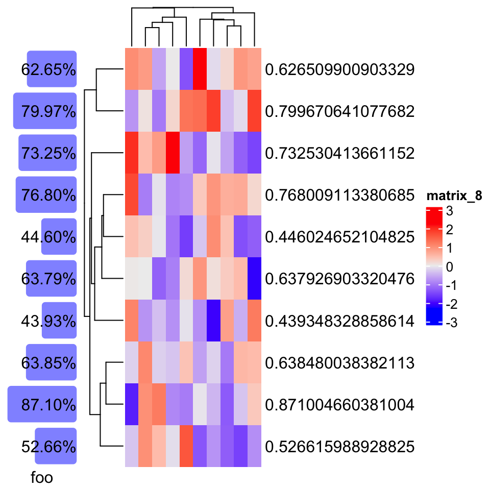

Note if cell_fun is set in AnnotationFunction, the returned annotation function is subsettable, which means it also works when heatmap is split.