6 GSEA framework
6.1 Overview
Recall in Chapter xx when we introduce the GSEA algorithm, the first step is to calcualte gene-level scores, then the gene-levels scores in a gene set is aggregated into a gene set-level score for testing. This procedure can be generalized into a general framework which includes calculation of gene level scores , gene set level scores and constructin of null distributions. According to how set-level statistic is designed, there are two main methologies: 1. univariate methods and 2. multivariate methods. where the first one is more used in current studies and the second one considered gene-gene correlation structures…
There are seveal reivews on the xxx.
6.2 The univariate methods
THe univariate methods is a two-step methods where the expression matrix is first merged into a gene-level scores which measures the gene-level differential expression. Later for each gene set, the member genes are merged into a single statistic where the permutation test is applied to construct the null distribution.
In two steps, the gene-gene correlation strucutre is actually not taken into consideration, thus it follows the univriate procedure where no co-variants are considered.
6.2.1 Gene-level methods
The first step of the univarirate procedures is to calculate the gene-level statistic, again, to make the discussion simple, we assume the data is from a two-condition comparison. and later we will demonstrate more complicated experimental designs. Let’s denote \(\mathbf{x_1}\) as the vector of gene expression for gene \(i\) in group 1, and \(\mathbf{x_2}\) as the vector of gene expression for gene \(i\) in group 2. The gene-level transformation is a function \(f()\) which applies on \(\mathbf{x_1}\) and \(\mathbf{x_2}\) togenerate a single value:
\[ f(\mathbf{x_1}, \mathbf{x_1}) -> a single value \]
There are variaty of methods that can be used to calculate gene-level scores. The only thing is that the score measures the degree of differnetial expression, thus high the absolute value of the score, more differnetial the gene is expressed. Commonly used methods are:
- t-value, defined as \(\frac{}{}\).
- log2 fold change
- signal-to-noise ratio
- SAM regularized t-values
In xxx, lists more gene-level statistics. However, the authors demonstarted the selection of gene-level statistic is less important for GSEA. The main reason is the method is always applied to the two vectors and without extra information, they performs similar. but still there are difference between various methods.
– scater plot
More generally, the relation between gene expression and the condition design can be modeled via linear regression. With linear regression, we can deal with more complicated experimental designs, such as 1. conditions with more than 2, 2. with continouse conditions e.g. age or dose treatment, 3. time series data, 4 multiple condition variates and 5. it allows a full model vs a reduced model to test the partial effect of a variate. For univariet,
\[y = \mu + \beta x + \epsilon \]
where \(x\) is the condition variable, which can be categorical variable, continuous variable or time series variable. Or with multiple variates:
\[ y = \mu + \beta_1 x_1 + \beta_2 x_2 + ... + \epsilon \]
The gene-level statistic can use the regression coeffcient to other statistics which measures the goodness of the liear fitting. However, users need to be careful that more complex models make the results less explainable.
6.2.2 Transformation of gene-level statistics
This step is optional and can be merged in to the previous step. With obtaining a vector of gene-level scores, we can apply proper transformation to it. The transformation is also a function which takes the original gene-level scores in and it outputs a new gene-level scores. There are the followng four widel y used transformations
- absolute
- square or power
- binary
- rank
The absolute or square transformation helps to capture the bi-directional changes and the square transformation can addtionally increase the weight of more differetiaally expressed genes. Binary transformation corresponds to ORA analysis and rank transformaton is used in GSEA.
Please note, till now we haven’t used any information of gene sets. The calculation of gene-level statistics is independen of gene sets. It is just a processing of the original matrix, In other words, it is a transformation of the original \(n x m\) matrix to a \(n\) vector. and in the next step, genes for gene sets are extracted from this gene-level vectors to calcualte into a gene set level statistic.
6.2.3 Set-level methods
With gene-level scores calculated already, we can check whether genes in a gene sets are in general differnetial expressed. Regarding what to compare, ie. the background, there are the following two scenarios:
- only consider genes in the gene set, in this case, the “background” is that all genes are not differnetially expressed. If there is a function for calculating gene-set level scores, it only takes a vector as input, which is the gene-level scores for genes in the current gene set.
- COmpare genes in the gene set and genes not in the gene set. Now the background is other genes. In this case, the gene set level function takes two vectors as input.
The two scenarions actaully measures different things, of which users need to keep in mide when they use corresponding methods.
For the first case, where the gene set level statistic is only calcualted in the gene set, it basically measures the overall difference of genes in the gene set. It is a aggregation of gene-level statstis into a singl set0-level statistic. There are the following widely used methods:
- Sum / Mean
- Median
- Maxmean
Note genes in a gene set may also show bi-directional pattern, which is some genes are up-regulated and some are down-regulated. Sum/Mean/Median are good at measure one-direcitonal change, but bi-direcitional change wil be cancled, thus get a very small value. This problem can be fixed by first apply a absolute transformation on gene-level scores.
Maxmean method was proposed in xxx. It basically takes the max mean of positive vlaues and negative values.
For the second scenario where also compare to genes not in the gene set. Denote the gene-level statistis for genes in the set as \(r_1\) and not in the set as \(r_0\), teh set-level statistic measures the difference between \(r_1\) and \(r_0\). There are the following three methods:
- (weighted) KS statistic
- Wilcoxon-rank statistic
- 2x2 contigency table
wiht the two vectors of \(r_1\) and \(r_0\), normally non-paremetric statistics are used, but for some methods which assume the normality, parametric test such as t-test can be used. But …
The 2x2 contigen table for ORA analysis actually also compare genes in the set and genes not in the set.
It works better when the differential expression for genes not in the set are weak. However, when a data has huge number of genes that are differnetial expressed e.g. cancer vs normal. this method may give wrong conclusions. e.g. when a gene set is significant, reseachers may make the conclusion that the biological function for this gnee set is significantly altered, but actually it xxx
Finally, it is very flexible to design a set-level statistic. There is only one principle for that: higher the value, more differnetial the genes in the gene set are.
6.2.5 Implement ORA under univariate framework
The ORA can be implemented under teh univate framework. In the 2x2 contigency table, the numer of genes in the gene set \(n_{11}\) actually can be used as the set-level statistic becuase higher the \(n_{11}\), the more enriched xxx. Then to translate into the univariate framework, we have:
- gene-level statistics: p-value/FDR from the differential expression test
- gene-level transformation: binary by setting a cutoff where e.g. if FDR < 0.05, 1, else 0)
- set-level statistics: sum, which is \(n_{11}\)
Note here \(n_{11}\) only used genes in the gene set.
We also introduced using chi-square test on the 2x2 contigency table, Thus, the Chi-suqare statistic can be used as teh set-level statistic. being differnet fro the first ORA translation, the chi-square test acautally compares genes in the gene set and not in the gene set.
The third way is, in the begnining when we introduce what is the overpresentation, we simply defined a value which is the fraction of two ratios. That value can also be a set-level statitic. Note this statistics alsoused information of genes in the set and not in the set.
For xxx, the p-values is calculatd as the probability of being larger than or equal to the observed values. When the set-level statists is only for one-directional change, and to see the power of down-regulation. Users may need to perform a second aalyais which looks at the other tail of hte null distribution.
6.2.6 Null distribution of set-level statistics
Once we have the set-level statistic, we need to construct the null distribution of it for calculting p-values. depends on the methods, there are teh following three ways:
- exact distribution
- parametric distribution
- permutation-based distributino
hypergeometric distribution is the exact distribution for ORA, however, it is normally impossbiel to obtain exact distibutions. Also users recall the hypergeometrix distribution has strong conditions that genes are independenly to be differnetially expressed, which may not fit the real cases.
Parametrix distribution needs assumptions of the distribution whihc is normally normal distributions for univaraite framework, but xxx. THe most used is the permuation-based distribution which construct the distribution directly from the data.
6.2.7 Permutation-based distribution
The permutaion generates null distribution from data, by permuting the origial data set to destroy the dependencies between xx and xx. It is non-parametrix and has no assumption of proir distribion. ALso there are three permutation methods:
- permute by samples
- permute by genes
- permute by both dimensions
In general, permutation is a powerful method to generate null distribution and to calculate p-values. But sinde the distribution
The two permutations, although they all randomize the data, they actually correspond to two very different null hypotheses:
for sample permutation, It only looks at the genes in the geneset and the null hypothesis is:
gene expression are not related to the condition settings.
In xxx, it is termed as self-contained.
For the gene permutation, it compares genes in the gene set and genes not in the gene set. The null hypotheses is :
differential gene expression is the gene set are the same as genes outside of the set.
Users can imagien one is horizontal comparison and the other is vertical comparison.
The two permutations are all widely used in current tools, each one has its advantages and disadvanges. For sample permutation, the main advantages ae:
- the gene-gene correlation is kept
- THe permutation has a clear and real biological meaning
THe distadvantages are
- Each time, gene-level statistics need to be recalculated
- more sensitive, assume only one genes in the set are differnetially expressed, the whole gene set can be assessed as significant.
For the gene permutation. the advantage is
- the gene-level statistics can be repeated used. Or in other words, the calculation of gene-level scores can be separated from GSEA where the input can just be a gene-level score vector.
The disadvanges are:
- the permutaiton assumes independency of genes and gene-gene correlation in the gene set are broken
- null distribution has no clear biological meanings
- It may work better when gene set is small and most of genes have no diffenritla expression in thie whote dataset.
It would be interesting to compare the sample permutation and gene permutation with a realworld data. Here the P53 dataset which was used in the original GSEA paper where the two groups are P53 wild type and P53 mutant. We take the “P53 pathway” gene set" which are expected to be significant.
to compare … assume \(s\) is the set-level score calclated from the real data and \(s_{null}\) is a vector of length 1000 calculated from permutation by sample or by gene, to compare between different methods, we calculated a relative value:
\[ \frac{s - mean_null}{sd_null} \]
which is a relative distance fro s to the center of null distribution.
In general, sample permutation is more statistically pwoerful than gene-permutation.
6.3 The multivariate methods
A second framework is the multivariate methods which takes in matrix as a singl input and returns the xx. They basically consider the co-variance in the data.
Normally, multivaraite methods are complex. They use complicated statistic computations trying to etablish a statsitcal framwork and …
- globaltest
- GlobalANCOVA
- Hotelling’ T2 test
Since their parametric nature, they need to assumptions, someti
The basically idea of multivariate methods is to follow either the following two linear models:
\[ A = bC + e \] \[ C = bA + e \]
where \(A\) and \(C\) are both matrices. to solve the problem, we can use pricinpal componet regression, partially lease square regression or regulazeid linear regression.
6.4 Implementation of GSEA framework
library(CePa)
condition = read.cls("data/P53.cls", treatment = "MUT", control = "WT")$label
condition = factor(condition, levels = c("WT", "MUT"))

expr = read.gct("data/P53_collapsed_symbols.gct")
The process of (univariate) GSEA analysis:

So basically, the calculation of gene-level statistics and set-level statistics can be separated.
We will implement the three independent parts: \(f()\), \(f'()\) and \(g()\).
We first implement the function that calculates gene-level statistics. To make things simple, we assume the matrix is from a two-condition comparison.
input: an expresion matrix (with condition labels)
output: a vector of gene-level scores
method: (t-value, log2fc, …)
# implement t-values as gene-level stat
gene_level = function(mat, condition) {

  tdf = genefilter:rowttests(mat, factor(condition))
  stat = tdf$statistic
  return(stat)
}
library(matrixStats)
library(genefilter)

# -condition to be a factor
gene_level = function(mat, condition, method = "tvalue") {

    le = levels(condition)
    l_group1 = condition == le[1]
    l_group2 = !l_group1

    mat1 = mat[, l_group1, drop = FALSE]  # sub-matrix for condition 1
    mat2 = mat[, l_group2, drop = FALSE]  # sub-matrix for condition 2

    if(method == "log2fc") {
        stat = log2(rowMeans(mat1)/rowMeans(mat2))
    } else if(method == "s2n") {
        stat = (rowMeans(mat1) - rowMeans(mat2))/(rowSds(mat1) + rowSds(mat2))
    } else if(method == "tvalue") {
        stat = (rowMeans(mat1) - rowMeans(mat2))/sqrt(rowVars(mat1)/ncol(mat1) + rowVars((mat2)/ncol(mat2)))
    } else if(method == "sam") {
        s = sqrt(rowVars(mat1)/ncol(mat1) + rowVars((mat2)/ncol(mat2)))
        stat = (rowMeans(mat1) - rowMeans(mat2))/(s + quantile(s, 0.1))
    } else if(method == "ttest") {
        stat = rowttests(mat, factor(condition))$p.value
    } else {
        stop("method is not supported.")
    }

    return(stat)
}
s = gene_level(expr, condition, method = "s2n")The transformation on gene-level values can actually be integrated as a part of the calculation of gene-level values, i.e. \(f'(f())\) can also be thought as a gene-level statistic.
if the gene-level stat is p-values we need to set a cutoff of p to convert to 1/0
binarize() input: is the origial gene-level stat (e.g. p-value) ouput: the values are 1/0
binarize = function(x) ifelse(x < 0.05, 1, 0)
if the gene-level stat is log2fc
binarize = function(x) ifelse(abs(x) > 1, 1, 0)
gene_level = function(mat, condition, method = "tvalue", transform = "none",
  binarize = function(x) x) {

    le = levels(condition)
    l_group1 = condition == le[1]
    l_group2 = !l_group1

    mat1 = mat[, l_group1, drop = FALSE]
    mat2 = mat[, l_group2, drop = FALSE]

    if(method == "log2fc") {
        stat = log2(rowMeans(mat1)/rowMeans(mat2))
    } else if(method == "s2n") {
        stat = (rowMeans(mat1) - rowMeans(mat2))/(rowSds(mat1) + rowSds(mat2))
    } else if(method == "tvalue") {
        stat = (rowMeans(mat1) - rowMeans(mat2))/sqrt(rowVars(mat1)/ncol(mat1) + rowVars((mat2)/ncol(mat2)))
    } else if(method == "sam") {
        s = sqrt(rowVars(mat1)/ncol(mat1) + rowVars((mat2)/ncol(mat2)))
        stat = (rowMeans(mat1) - rowMeans(mat2))/(s + quantile(s, 0.1))
    } else if(method == "ttest") {
        stat = rowttests(mat, factor(condition))$p.value
    } else {
        stop("method is not supported.")
    }

    if(transform == "none") {

    } else if(transform == "abs") {
        stat = abs(stat)
    } else if(transform == "square") {
        stat = stat^2
    } else if(transform == "binary") {
        stat = binarize(stat)
    } else {
        stop("method is not supported.")
    }

    return(stat)
}
Let’s test gene_level(). Here we still use the p53 dataset which is from the GSEA original paper.
Let’s check the gene-level values:
methods = c("log2fc", "s2n", "tvalue", "sam")
lt = lapply(methods, function(x) gene_level(expr, condition, method = x))
names(lt) = methods
pairs(lt)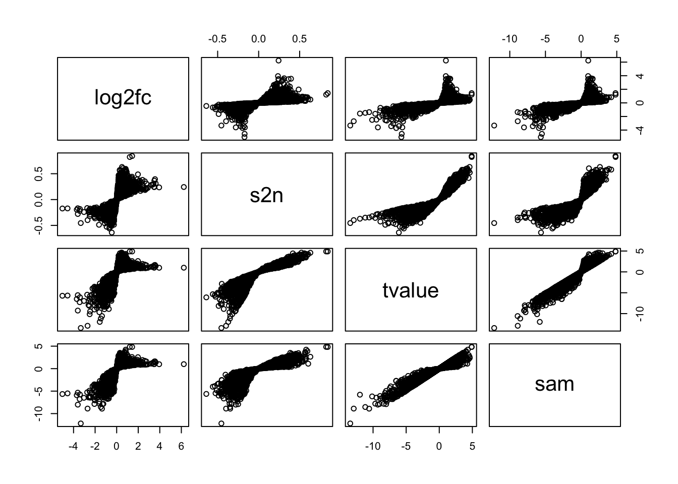
Also we can check number of differential genes (gene level: ttest + transform: binary).
Note a better way is to filter by FDR, but for simplicity, we use p-values directly.
s = gene_level(expr, condition, method = "ttest", transform = "binary",
    binarize = function(x) ifelse(x < 0.05, 1, 0))
table(s)
# s
#    0    1
# 9394  706
If method is set to log2fc, then the differential genes can be selected by setting a cutoff for log2 fold change.
s = gene_level(expr, condition, method = "log2fc", transform = "binary",
    binarize = function(x) ifelse(abs(x) > 1, 1, 0))
table(s)
# s
#    0    1
# 9717  383
Implementing gene_level() is actually simply.
Next we implement the calculation of set-level statistics. A nature design for the set-level function is to let it accept a vector of gene-level statistics and a gene set represented as a vector of genes, like follows:
set_fun = function(gene_stat, geneset) {
    s = gene_stat[geneset]
    mean(s)
}
However, we need to make sure all genes in geneset are also in gene_stat. A safer way
is to test which genes in gene_stat are also in geneset:
However, recall the set-level can also be calculated based on genes outside of the gene set. Thus the two arguments in set_level() are a vector of gene-level statistics for all genes and a logical vector which shows whether genes in the current gene set. In this setting, we can know both which genes are in the set and which genes are not in the set.
before geneset is a vector of gene IDs
now l_set: a logical vector, which has the same length of gene_stat,
if the value is TRUE, it means the gene is in the set, if it is FALSE, the gene is NOT in the set
set_level = function(gene_stat, l_set, method = "mean") {
    if(!any(l_set)) {
        return(NA)
    }

    if(method == "mean") {
        stat = mean(gene_stat[l_set])
    } else if(method == "sum") {
        stat = sum(gene_stat[l_set])
    } else if(method == "median") {
        stat = median(gene_stat[l_set])
    } else if(method == "maxmean") {
        s = gene_stat[l_set]
        s1 = mean(s[s > 0]) # s1 is positive
        s2 = mean(s[s < 0])  # s2 is negative
        stat = ifelse(s1 > abs(s2), s1, s2)
    } else if(method == "ks") {
        # order gene_stat
        od = order(gene_stat, decreasing = TRUE)
        gene_stat = gene_stat[od]
        l_set = l_set[od]

        s_set = abs(gene_stat)
        s_set[!l_set] = 0
        f1 = cumsum(s_set)/sum(s_set)

        l_other = !l_set
        f2 = cumsum(l_other)/sum(l_other)

        stat = max(f1 - f2)
    } else if(method == "wilcox") {
        stat = wilcox.test(gene_stat[l_set], gene_stat[!l_set])$statistic
    } else if(method == "chisq") {
        # should on work with binary gene-level statistics
        stat = chisq.test(factor(gene_stat), factor(as.numeric(l_set)))$statistic
    } else {
        stop("method is not supported.")
    }

    return(stat)
}
Let’s check set_level():
input of set_level():
- a gene-level scores
- a logical vector which shows whether the genes are in a set
gene_stat = gene_level(expr, condition)

ln = strsplit(readLines("data/c2.symbols.gmt"), "\t")
gs = lapply(ln, function(x) x[-(1:2)])
names(gs) = sapply(ln, function(x) x[1])

geneset = gs[["p53hypoxiaPathway"]]
l_set = rownames(expr) %in% geneset
set_level(gene_stat, l_set)
# [1] 0.8476668
set_level(gene_stat, l_set, method = "ks")
# [1] 0.6380268
Now we can wrap gene_level() and set_level() into a single function gsea_tiny() which accepts the expression and one gene set as input,
and it returns the set-level score.
gsea_tiny():
- expression matrix (condition labels)
- a gene set
output: a set-level statistic
gsea_tiny() [ gene_level() + set_level() ]
gsea_tiny = function(mat, condition,
    gene_level_method = "tvalue", transform = "none", binarize = function(x) x,
    set_level_method = "mean", geneset) {

    gene_stat = gene_level(mat, condition, method = gene_level_method,
        transform = transform, binarize = binarize)

    l_set = rownames(mat) %in% geneset

    set_stat = set_level(gene_stat, l_set, method = set_level_method)

    return(set_stat)
}
We apply gsea_tiny() to the p53 dataset.
gsea_tiny(expr, condition, geneset = geneset)
# [1] 0.8476668
We use wilcox.test() to calculate the Wilcoxon statistic. Note this function also does a lot of extra calculations. We can implement a function which “just” calculates the Wilcoxon statistic but do nothing else:
The formula is from Wikipedia (https://en.wikipedia.org/wiki/Mann%E2%80%93Whitney_U_test).
Note, to make wilcox_stat() faster, we only use maximal 100 data points. It is only
for demonstration purpose, you should not use it in real applications.
“outer” calculation
x, y every value in x to every value in y
if length(x) is n, length(y) is m
n*m
m = outer(x, y, “>”)
wilcox_stat = function(x1, x2) {
  if(length(x1) > 100) {
    x1 = sample(x1, 100)
  }
  if(length(x2) > 100) {
    x2 = sample(x2, 100)
  }
  sum(outer(x1, x2, ">"))
}
Similarly, we implement a new function which only calculates chi-square statistic:
# x1: a logical vector or a binary vector
# x2: a logical vector or a binary vector
chisq_stat = function(x1, x2) {
    n11 = sum(x1 & x2)
    n10 = sum(x1)
    n20 = sum(!x1)
    n01 = sum(x2)
    n02 = sum(!x2)
    n = length(x1)

    n12 = n10 - n11
    n21 = n01 - n11
    n22 = n20 - n21

    p10 = n10/n
    p20 = n20/n
    p01 = n01/n
    p02 = n02/n

    e11 = n*p10*p01
    e12 = n*p10*p02
    e21 = n*p20*p01
    e22 = n*p20*p02

    stat = (n11 - e11)^2/e11 +
           (n12 - e12)^2/e12 +
           (n21 - e21)^2/e21 +
           (n22 - e22)^2/e22
    return(stat)
}
and we change set_level() accordingly:
set_level = function(gene_stat, l_set, method = "mean") {
    if(!any(l_set)) {
        return(NA)
    }

    if(method == "mean") {
        stat = mean(gene_stat[l_set])
    } else if(method == "sum") {
        stat = sum(gene_stat[l_set])
    } else if(method == "median") {
        stat = median(gene_stat[l_set])
    } else if(method == "maxmean") {
        s = gene_stat[l_set]
        s1 = mean(s[s > 0])
        s2 = mean(s[s < 0])
        stat = ifelse(s1 > abs(s2), s1, s2)
    } else if(method == "ks") {
        # order gene_stat
        od = order(gene_stat, decreasing = TRUE)
        gene_stat = gene_stat[od]
        l_set = l_set[od]

        s_set = abs(gene_stat)
        s_set[!l_set] = 0
        f1 = cumsum(s_set)/sum(s_set)

        l_other = !l_set
        f2 = cumsum(l_other)/sum(l_other)

        stat = max(f1 - f2)
    } else if(method == "wilcox") {
        stat = wilcox_stat(gene_stat[l_set], gene_stat[!l_set])
    } else if(method == "chisq") {
        # should on work with binary gene-level statistics
        stat = chisq_stat(gene_stat, l_set)
    } else {
        stop("method is not supported.")
    }

    return(stat)
}
Next we will adjust gsea_tiny() to let it work for multiple gene sets and support random permutation for p-value calculation.
To let is support a list of gene sets, simply change the format of geneset variable.
6.5 geneset to be a list of gene sets
# geneset: a list of vectors (gene IDs)
gsea_tiny = function(mat, condition,
    gene_level_method = "tvalue", transform = "none", binarize = function(x) x,
    gene_stat, set_level_method = "mean", geneset) {

    gene_stat = gene_level(mat, condition, method = gene_level_method,
        transform = transform, binarize = binarize)

    set_stat = sapply(geneset, function(set) {
        l_set = rownames(mat) %in% set

        set_level(gene_stat, l_set, set_level_method)
    })

    return(set_stat)
}
Check the new version of gsea_tiny():
ss = gsea_tiny(expr, condition, geneset = gs)
head(ss)
#          41bbPathway          ace2Pathway acetaminophenPathway
#           -0.3125486            1.2710342            0.3441254
#           achPathway
#           -0.2944815
Now with gsea_tiny(), we can also generate the null distribution of the set-level statistics, just by
generating random matrices.
# sample permutation
ss_random = list()
for(i in 1:1000) {
    ss_random[[i]] = gsea_tiny(mat, sample(condition), geneset = gs)
}

# or gene permutation
for(i in 1:1000) {
    mat2 = mat
    rownames(mat2) = sample(rownames(mat))
    ss_random[[i]] = gsea_tiny(mat2, condition, geneset = gs)
}
A better design is to integrate permutation procedures inside gsea_tiny(). We first integrate sample permutation:
gsea_tiny = function(mat, condition,
    gene_level_method = "tvalue", transform = "none", binarize = function(x) x,
    gene_stat, set_level_method = "mean", geneset,
    nperm = 1000) {

    gene_stat = gene_level(mat, condition, method = gene_level_method,
        transform = transform, binarize = binarize)

    set_stat = sapply(geneset, function(set) {
        l_set = rownames(mat) %in% set

        set_level(gene_stat, l_set, set_level_method)
    })

    ## null distribution
    set_stat_random = list()

    for(i in seq_len(nperm)) {
        condition2 = sample(condition)
        gene_stat = gene_level(mat, condition2, method = gene_level_method,
            transform = transform, binarize = binarize)

        set_stat_random[[i]] = sapply(geneset, function(set) {
            l_set = rownames(mat) %in% set

            set_level(gene_stat, l_set, set_level_method)
        })

        if(i %% 100 == 0) {
            message(i, " permutations done.")
        }
    }

    set_stat_random = do.call(cbind, set_stat_random)

    n_set = length(geneset)
    p = numeric(n_set)
    for(i in seq_len(n_set)) {
        p[i] = sum(set_stat_random[i, ] >= set_stat[i])/nperm
    }

    # the function returns a data frame
    df = data.frame(stat = set_stat,
                    size = sapply(geneset, length),
                    p.value = p)
    df$fdr = p.adjust(p, "BH")

    return(df)
}
Let’s have a try. It is actually quite slow to run 1000 permutations.
df = gsea_tiny(expr, condition, geneset = gs)This is the basic procedures of developing new R functions. First we make sure the functions are working, next we optimize the functions to let them running faster or use less memory.
gsea_tiny() running with 100 permutations only needs several seconds.
df = gsea_tiny(expr, condition, geneset = gs, nperm = 100)The package profvis provides an easy to for profiling.
We can see the process of %in% uses quite a lot of running time.
we can first calculate the relations of genes and sets and later they can be repeatedly used.
gsea_tiny = function(mat, condition,
    gene_level_method = "tvalue", transform = "none", binarize = function(x) x,
    gene_stat, set_level_method = "mean", geneset,
    nperm = 1000) {

    gene_stat = gene_level(mat, condition, method = gene_level_method,
        transform = transform, binarize = binarize)

    # now this only needs to be calculated once
    l_set_list = lapply(geneset, function(set) {
        rownames(mat) %in% set
    })

    set_stat = sapply(l_set_list, function(l_set) {
        set_level(gene_stat, l_set, set_level_method)
    })

    ## null distribution
    set_stat_random = list()

    for(i in seq_len(nperm)) {
        condition2 = sample(condition)
        gene_stat_random = gene_level(mat, condition2, method = gene_level_method,
            transform = transform, binarize = binarize)

        # here we directly use l_set_list
        set_stat_random[[i]] = sapply(l_set_list, function(l_set) {
            set_level(gene_stat_random, l_set, set_level_method)
        })

        if(i %% 100 == 0) {
            message(i, " permutations done.")
        }
    }

    set_stat_random = do.call(cbind, set_stat_random)

    n_set = length(geneset)
    p = numeric(n_set)
    for(i in seq_len(n_set)) {
        p[i] = sum(set_stat_random[i, ] >= set_stat[i])/nperm
    }

    df = data.frame(stat = set_stat,
                    size = sapply(geneset, length),
                    p.value = p)
    df$fdr = p.adjust(p, "BH")

    return(df)
}
Now it is faster for 1000 permutations:
df = gsea_tiny(expr, condition, geneset = gs)To support gene permutation, we only need to permute the gene-level statistics calculated from the original matrix.
Note we also move position of geneset argument to the start of the argument list because it is a must-set argument.
gsea_tiny = function(mat, condition, geneset,
    gene_level_method = "tvalue", transform = "none", binarize = function(x) x,
    gene_stat, set_level_method = "mean",
    nperm = 1000, perm_type = "sample") {

    gene_stat = gene_level(mat, condition, method = gene_level_method,
        transform = transform, binarize = binarize)
    l_set_list = lapply(geneset, function(set) {
        rownames(mat) %in% set
    })

    set_stat = sapply(l_set_list, function(l_set) {
        set_level(gene_stat, l_set, set_level_method)
    })

    ## null distribution
    set_stat_random = list()

    for(i in seq_len(nperm)) {

        if(perm_type == "sample") {
            condition2 = sample(condition)
            gene_stat_random = gene_level(mat, condition2, method = gene_level_method,
                transform = transform, binarize = binarize)

            set_stat_random[[i]] = sapply(l_set_list, function(l_set) {
                set_level(gene_stat_random, l_set, set_level_method)
            })
        } else if(perm_type == "gene") {
            gene_stat_random = sample(gene_stat)

            set_stat_random[[i]] = sapply(l_set_list, function(l_set) {
                set_level(gene_stat_random, l_set, set_level_method)
            })
        } else {
            stop("wrong permutation type.")
        }

        if(i %% 100 == 0) {
            message(i, " permutations done.")
        }
    }

    set_stat_random = do.call(cbind, set_stat_random)

    n_set = length(geneset)
    p = numeric(n_set)
    for(i in seq_len(n_set)) {
        p[i] = sum(set_stat_random[i, ] >= set_stat[i])/nperm
    }

    df = data.frame(stat = set_stat,
                    size = sapply(geneset, length),
                    p.value = p)
    df$fdr = p.adjust(p, "BH")

    return(df)
}
Let’s check:
set.seed(123)
df1 = gsea_tiny(expr, condition, geneset = gs, perm_type = "sample")
df2 = gsea_tiny(expr, condition, geneset = gs, perm_type = "gene")
df1 = df1[order(df1$p.value), ]
df2 = df2[order(df2$p.value), ]
head(df1)
#                        stat size p.value fdr
# hsp27Pathway      1.1077565   16       0   0
# p53hypoxiaPathway 0.8476668   20       0   0
# p53Pathway        1.1781147   16       0   0
# HTERT_DOWN        0.3002211   67       0   0
head(df2)
#                    stat size p.value fdr
# ace2Pathway   1.2710342   12       0   0
# inflamPathway 0.7852193   29       0   0
# p53Pathway    1.1781147   16       0   0
# P53_UP        0.9864715   40       0   0
Note, above settings can only detect the up-regulated gene sets.
Great! If we think each combination of gene-level method, gene-level transformation and set-level method is a GSEA method, then our gsea_tiny() actually already support many GSEA methods! The whole functionality only contains 180 lines of code (https://gist.github.com/jokergoo/e8fff4a57ec59efc694b9e730da22b9f).
6.6 current tools for GSEA framework
Package EnrichmentBrowser integrates a lot of GSEA methods. The integrated methods are:
library(EnrichmentBrowser)
sbeaMethods()
#  [1] "ora"        "safe"       "gsea"       "gsa"        "padog"
#  [6] "globaltest" "roast"      "camera"     "gsva"       "samgs"
# [11] "ebm"        "mgsa"
EnrichmentBrowser needs a special format (in SummarizedExperiment) as input.
Condition labels should be stored in a column “GROUP.” Log2 fold change and adjusted p-values should be saved in “FC” and “ADJ.PVAL” columns.
library(CePa)
condition = read.cls("data/P53.cls", treatment = "MUT", control = "WT")$label
expr = read.gct("data/P53_collapsed_symbols.gct")


library(SummarizedExperiment)
se = SummarizedExperiment(assays = SimpleList(expr = expr))
colData(se) = DataFrame(GROUP = ifelse(condition == "WT", 1, 0))

l = condition == "WT"

library(genefilter)
tdf = rowttests(expr, factor(condition))
rowData(se) = DataFrame(FC = log2(rowMeans(expr[, l])/rowMeans(expr[, !l])),
                        ADJ.PVAL = p.adjust(tdf$p.value))
se
# class: SummarizedExperiment
# dim: 10100 50
# metadata(0):
# assays(1): expr
# rownames(10100): TACC2 C14orf132 ... AMACR LDLR
# rowData names(2): FC ADJ.PVAL
# colnames: NULL
# colData names(1): GROUP
Note, to run eaBrowse(), you need to explicitly convert to ENTREZID.
se = idMap(se, org = "hsa", from = "SYMBOL", to = "ENTREZID") # !! Gene ID must be converted to EntrezIDWe load the hallmark gene sets by package msigdbr.
When using the Entrez ID, make sure the “numbers” are converted to “characters.”
library(msigdbr)
gs = msigdbr(category = "H")
gs = split(gs$human_entrez_gene, gs$gs_name)  # Entrez ID must be used
gs = lapply(gs, as.character)                 # be careful Entrez ID might be wrongly used as integers, convert them into characters
Simply call sbea() function with a specific method:
Note now you can use eaBowse(res) to create the tiny website for detailed results.
Next we run all supported GSEA methods in EnrichmentBrowser.
all_gsea_methods = sbeaMethods()
all_gsea_methods
#  [1] "ora"        "safe"       "gsea"       "gsa"        "padog"
#  [6] "globaltest" "roast"      "camera"     "gsva"       "samgs"
# [11] "ebm"        "mgsa"
all_gsea_methods = setdiff(all_gsea_methods, "padog")
res_list = lapply(all_gsea_methods, function(method) {
sbea(method = method, se = se, gs = gs)
})
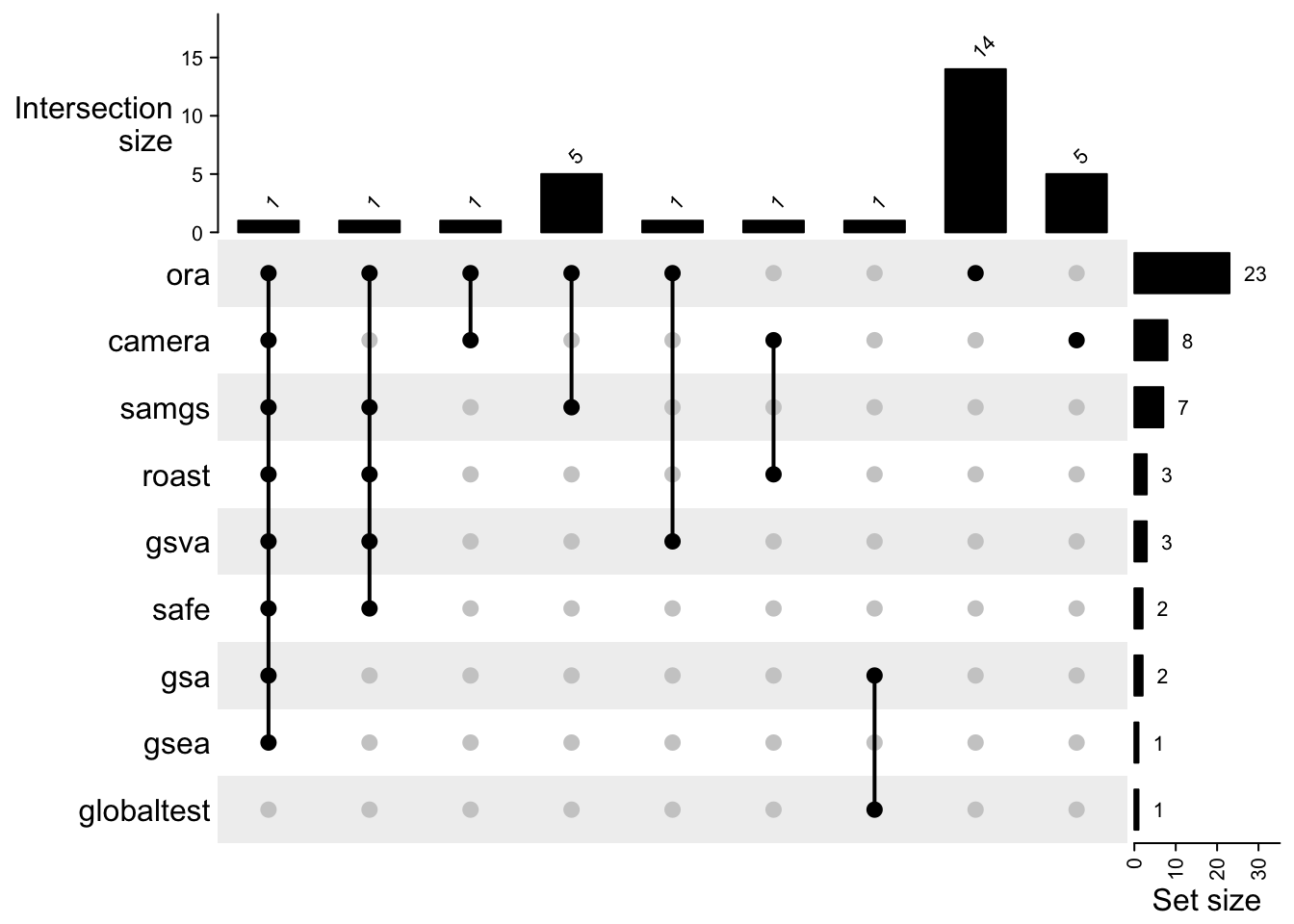
names(res_list) = all_gsea_methodsWe compare the significant gene sets from different methods.
tb_list = lapply(res_list, gsRanking)
tb_list
# $ora
# DataFrame with 23 rows and 4 columns
#                   GENE.SET GLOB.STAT NGLOB.STAT      PVAL
#                <character> <numeric>  <numeric> <numeric>
# 1     HALLMARK_P53_PATHWAY         2    0.01480     0.001
# 2       HALLMARK_APOPTOSIS         2    0.01420     0.001
# 3   HALLMARK_PI3K_AKT_MT..         1    0.01250     0.001
# 4   HALLMARK_INTERFERON_..         1    0.00730     0.001
# 5      HALLMARK_MYOGENESIS         1    0.00592     0.002
# ...                    ...       ...        ...       ...
# 19  HALLMARK_REACTIVE_OX..         0          0     0.023
# 20  HALLMARK_INTERFERON_..         0          0     0.026
# 21  HALLMARK_TGF_BETA_SI..         0          0     0.029
# 22  HALLMARK_ANDROGEN_RE..         0          0     0.039
# 23  HALLMARK_CHOLESTEROL..         0          0     0.044
#
# $safe
# DataFrame with 2 rows and 4 columns
#                 GENE.SET GLOB.STAT NGLOB.STAT      PVAL
#              <character> <numeric>  <numeric> <numeric>
# 1   HALLMARK_P53_PATHWAY    225000       1660     0.021
# 2 HALLMARK_HEDGEHOG_SI..     51300       1830     0.033
#
# $gsea
# DataFrame with 1 row and 4 columns
#               GENE.SET        ES       NES      PVAL
#            <character> <numeric> <numeric> <numeric>
# 1 HALLMARK_P53_PATHWAY     0.355       1.5    0.0421
#
# $gsa
# DataFrame with 2 rows and 3 columns
#                 GENE.SET     SCORE      PVAL
#              <character> <numeric> <numeric>
# 1   HALLMARK_P53_PATHWAY     0.388     0.012
# 2 HALLMARK_IL6_JAK_STA..     0.455     0.020
#
# $globaltest
# DataFrame with 1 row and 3 columns
#                 GENE.SET      STAT      PVAL
#              <character> <numeric> <numeric>
# 1 HALLMARK_IL6_JAK_STA..      4.41     0.008
#
# $roast
# DataFrame with 3 rows and 4 columns
#                 GENE.SET  NR.GENES       DIR      PVAL
#              <character> <numeric> <numeric> <numeric>
# 1   HALLMARK_P53_PATHWAY       135         1  0.000999
# 2 HALLMARK_ALLOGRAFT_R..       168         1  0.038000
# 3 HALLMARK_HEDGEHOG_SI..        28         1  0.040000
#
# $camera
# DataFrame with 8 rows and 4 columns
#                 GENE.SET  NR.GENES       DIR      PVAL
#              <character> <numeric> <numeric> <numeric>
# 1 HALLMARK_G2M_CHECKPO..       142        -1  0.000412
# 2 HALLMARK_ALLOGRAFT_R..       168         1  0.000824
# 3   HALLMARK_E2F_TARGETS       129        -1  0.001960
# 4 HALLMARK_MITOTIC_SPI..       116        -1  0.011800
# 5   HALLMARK_P53_PATHWAY       135         1  0.014700
# 6 HALLMARK_PROTEIN_SEC..        80        -1  0.022000
# 7 HALLMARK_KRAS_SIGNAL..       124         1  0.022900
# 8 HALLMARK_UV_RESPONSE..       122        -1  0.028800
#
# $gsva
# DataFrame with 3 rows and 3 columns
#                 GENE.SET   t.SCORE      PVAL
#              <character> <numeric> <numeric>
# 1 HALLMARK_WNT_BETA_CA..     -2.12    0.0389
# 2 HALLMARK_HEDGEHOG_SI..      2.12    0.0390
# 3   HALLMARK_P53_PATHWAY      2.06    0.0445
#
# $samgs
# DataFrame with 7 rows and 4 columns
#                 GENE.SET SUMSQ.STAT NSUMSQ.STAT      PVAL
#              <character>  <numeric>   <numeric> <numeric>
# 1   HALLMARK_P53_PATHWAY        322        2.38     0.000
# 2     HALLMARK_APOPTOSIS        257        1.83     0.003
# 3 HALLMARK_HEDGEHOG_SI..         50        1.78     0.012
# 4    HALLMARK_MYOGENESIS        245        1.45     0.017
# 5 HALLMARK_INTERFERON_..        209        1.52     0.024
# 6 HALLMARK_INFLAMMATOR..        218        1.36     0.025
# 7 HALLMARK_TNFA_SIGNAL..        226        1.44     0.041
#
# $ebm
# NULL
#
# $mgsa
# NULL
tb_list = tb_list[sapply(tb_list, length) > 0]

library(ComplexHeatmap)
cm = make_comb_mat(lapply(tb_list, function(x) x[[1]]))
UpSet(cm,
    top_annotation = upset_top_annotation(cm, add_numbers = TRUE),
    right_annotation = upset_right_annotation(cm, add_numbers = TRUE)
)
6.7 Important aspects of GSEA methogology
Sample size is a general factor of stastics where more samples give more pwoer for the statistical tests.
Gene sets have differnet sizes. it will affect teh null distribution (mostly the standard deviation) of set-level statistic
In ORA, it assumes genes are independent, also in some parametric methods, after xxx, which also assume … However, ignore the gene correlation will, moslty estimate the wrong varaince. Nevertheless, we suggest to use sample permutation which keeps the gene correlation structure during the xxx
6.8 recommandations of methods
Due to the test is a information reduction from a matrix to a sigle value,
- use GSEA method
- use sample permutation
- use self-contained setlevel
- use simply model
Additionally, which is also recommneded for general data ananlysis, explorrary data anlaysi (EDA) should be first applied to the , eg.. to check the global direrential expression, which helps to find a proper method.
If you only have a list of genes, then use ORA with hypergeometric distribution and set whole protaincoding genes as background
If you have a vector of pre-computed gene-level scores, use GSEA tool with gene-permutation version. ANd it suggested to first check the global distribution of gene level scores…
If yo uhave a complete matrix, then use GSEA with sample permutations