Benchmark

Prepare

The function unique_strings() generates a vector of unique strings. It simply uses digest package to generate MD5 hashes of R objects (in the following example, hashed R objects are integers).

library(hashtable)
library(microbenchmark)
library(digest)
unique_strings = function(k) {
    sapply(seq_len(k), digest)
}
unique_strings(2)

## [1] "4b5630ee914e848e8d07221556b0a2fb" "c01f179e4b57ab8bd9de309e6d576c48"

bm() is only for simplifying code demo in this document.

bm = function(...) {
    mean(microbenchmark(..., times = 50)$time)
}

There are the following packages implementing hash tables:

hash, using environment,
hashmapR, using C++ library std::unordered_map,
r2r, using environment.

There are also other indirect hash table implementations:

list2env(), converting a list to an environment.
fastmatch, matching between two character vectors where a hash table is internally computated and attached to one character vector.

We compare the performance of creating, querying, deleting and inserting keys of hashtable and other methods.

Create hash tables

There are three implementations of hash tables in hashtable:

hash_table(), using C++ library std::unordered_map,
hash_fm_table(), using fastmatch,
hash_env_table(), using environment.

We test hash tables with size from 10K keys to 100K keys.

size = seq(10000L, 100000L, by = 10000L)

list2env() expects the input as a named list. hashmapR::hashmap() expects keys and values both specified as lists. r2r::hashmap() creates the hash table in two steps: create an empty object then fill key-value pairs. Note format preparation is not included in estimating runtime of benchmarking functions.

t1 = t2 = t3 = t4 = t5 = t6 = t7 = numeric(length(size))
for(i in seq_along(size)) {
    keys = unique_strings(size[i])
    values = seq_len(size[i])

    t1[i] = bm(hash_table(keys = keys, values = values))
    t2[i] = bm(hash_fm_table(keys = keys, values = values))
    t3[i] = bm(hash_env_table(keys = keys, values = values))
    
    lt = split(values, keys)
    t4[i] = bm(list2env(lt, hash = TRUE, parent = emptyenv()))
    t5[i] = bm(hash::hash(keys = keys, values = values))

    lt_keys = split(keys, keys)
    lt_values = split(values, keys)
    t6[i] = bm({h = hashmapR::hashmap(); h$set(lt_keys, lt_values, vectorize = TRUE)})
    t7[i] = bm({h = r2r::hashmap(); h[keys] = values})
}
matplot(size, cbind(t1, t2, t3, t4, t5, t6, t7)/1000, type = "o", 
    lty = 1, col = 1:7, pch = 16, cex = 0.5, 
    xlab = "size", ylab = "microseconds", main = "Create hash tables")
legend("topleft", lty = 1, col = 1:7, 
    legend = c("hash_table", "hash_fm_table", "hash_env_table", "list2env", "hash", "hashmapR", "r2r"))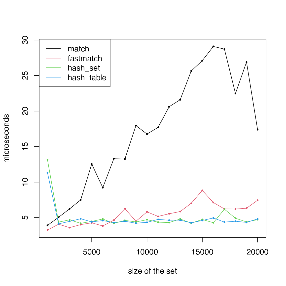

Obviously, hashtable is the fastest to create hash tables.

Query

Query a single key. Except hashmapR, all hash table objects created by various methods support [[ index to get a single value.

t1 = t2 = t3 = t4 = t5 = t6 = t7 = numeric(length(size))
for(i in seq_along(size)) {
    keys = unique_strings(size[i])
    values = seq_along(keys)

    h1 = hash_table(keys = keys, values = values)
    h2 = hash_fm_table(keys = keys, values = values)
    h3 = hash_env_table(keys = keys, values = values)
    
    lt = split(values, keys)
    h4 = list2env(lt, hash = TRUE, parent = emptyenv())

    h5 = hash::hash(keys = keys, values = values)
    
    h6 = hashmapR::hashmap()
    h6$set(split(keys, keys), split(values, keys), vectorize = TRUE)

    h7 = r2r::hashmap()
    h7[keys] = values

    t1[i] = bm(h1[[sample(keys, 1)]])
    t2[i] = bm(h2[[sample(keys, 1)]])
    t3[i] = bm(h3[[sample(keys, 1)]])
    t4[i] = bm(h4[[sample(keys, 1)]])
    t5[i] = bm(h5[[sample(keys, 1)]])
    t6[i] = bm(h6$get(sample(keys, 1)))
    t7[i] = bm(h7[[sample(keys, 1)]])
}
matplot(size, cbind(t1, t2, t3, t4, t5, t6, t7)/1000, type = "o", 
    lty = 1, col = 1:7, pch = 16, cex = 0.5, 
    xlab = "size", ylab = "microseconds", main = "Query a single key")
legend("topleft", lty = 1, col = 1:7, 
    legend = c("hash_table", "hash_fm_table", "hash_env_table", "list2env", "hash", "hashmapR", "r2r"))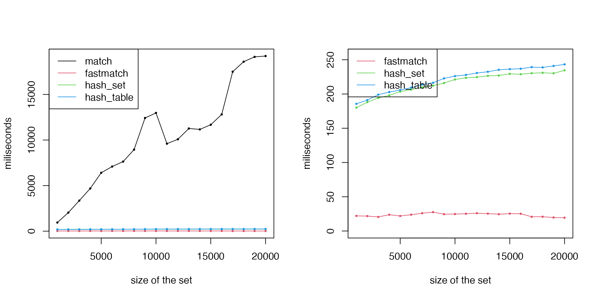

All hash-functions have similar performance. The small difference of runtime is due to their specific implementations, e.g., hashtable implements functions using S4, so it needs a little bit more steps on method dispatch.

Query multiple keys. We use mget() to get multiple values from an environment. Many methods support [ index to get multiple values.

par(mfrow = c(2, 2))
for(p in c(0.01, 0.1, 0.25, 0.5)) {
    t1 = t2 = t3 = t4 = t5 = t6 = t7 = numeric(length(size))
    for(i in seq_along(size)) {
        keys = unique_strings(size[i])
        values = seq_along(keys)

        h1 = hash_table(keys = keys, values = values)
        h2 = hash_fm_table(keys = keys, values = values)
        h3 = hash_env_table(keys = keys, values = values)
        
        lt = split(values, keys)
        h4 = list2env(lt, hash = TRUE, parent = emptyenv())

        h5 = hash::hash(keys = keys, values = values)
        
        h6 = hashmapR::hashmap()
        h6$set(split(keys, keys), split(values, keys), vectorize = TRUE)

        h7 = r2r::hashmap()
        h7[keys] = values

        nk = round(p*size[i])
        t1[i] = bm(h1[sample(keys, nk)])
        t2[i] = bm(h2[sample(keys, nk)])
        t3[i] = bm(h3[sample(keys, nk)])
        t4[i] = bm(mget(sample(keys, nk), h4))
        t5[i] = bm(h5[sample(keys, nk)])
        t6[i] = bm(h6$get(sample(keys, nk)))
        t7[i] = bm(h7[sample(keys, nk)])
    }
    matplot(size, cbind(t1, t2, t3, t4, t5, t6, t7)/1000, type = "o", 
        lty = 1, col = 1:7, pch = 16, cex = 0.5, 
        xlab = "size", ylab = "microseconds", main = paste0("Query multiple keys, ", p*100, "%"))
    legend("topleft", lty = 1, col = 1:7, 
        legend = c("hash_table", "hash_fm_table", "hash_env_table", "list2env", "hash", "hashmapR", "r2r"))
}

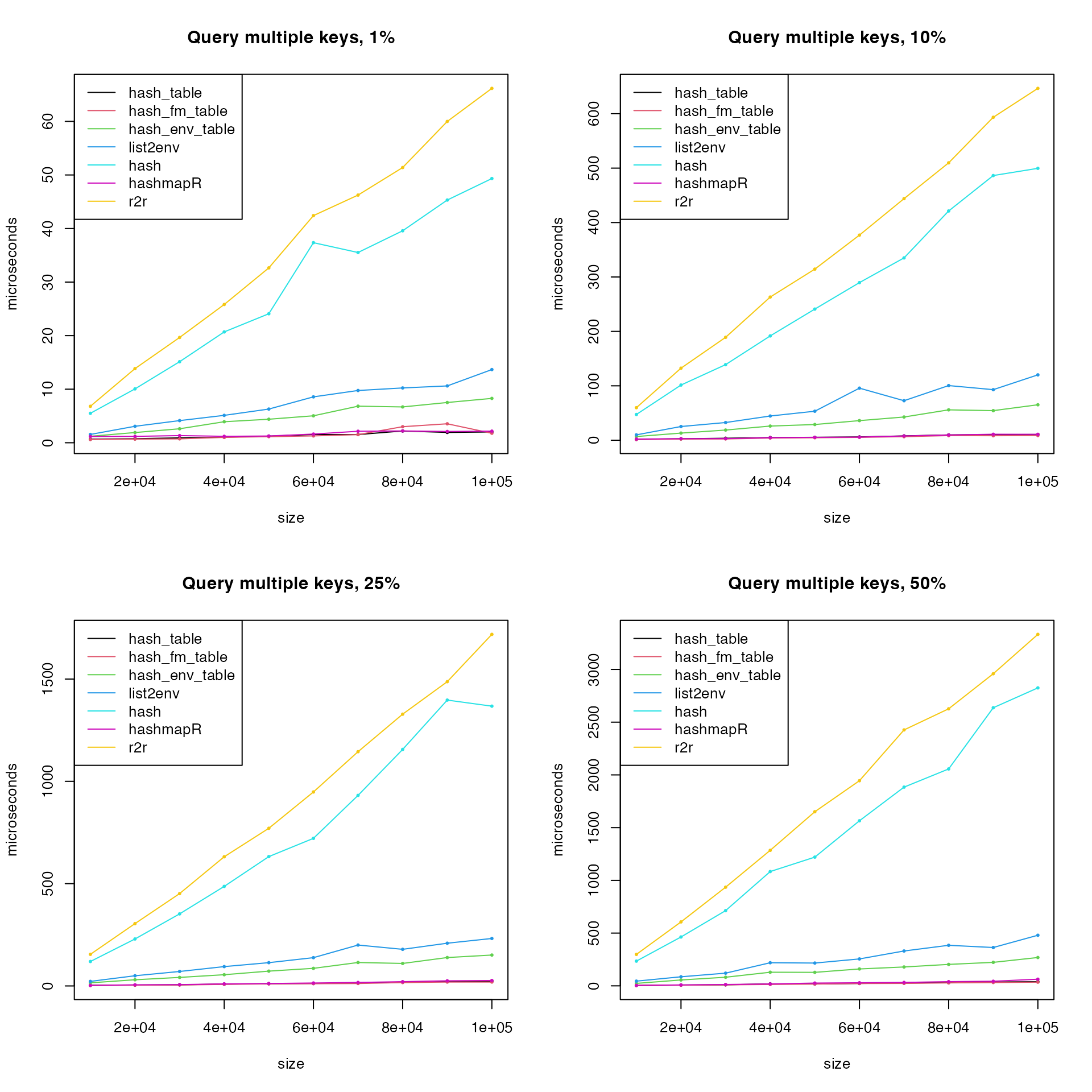
r2r and hash performs badly when querying multiple keys. Remove r2r, hash() also remove two environment-functions list2env() and hash_env_table(), then remake the last plot:

matplot(size, cbind(t1, t2, t6)/1000, type = "o", 
    lty = 1, col = c(1:2, 6), pch = 16, cex = 0.5, 
    xlab = "size", ylab = "microseconds", main = paste0("Query multiple keys, ", p*100, "%"))
legend("topleft", lty = 1, col = c(1:2, 6), 
    legend = c("hash_table", "hash_fm_table", "hashmapR"))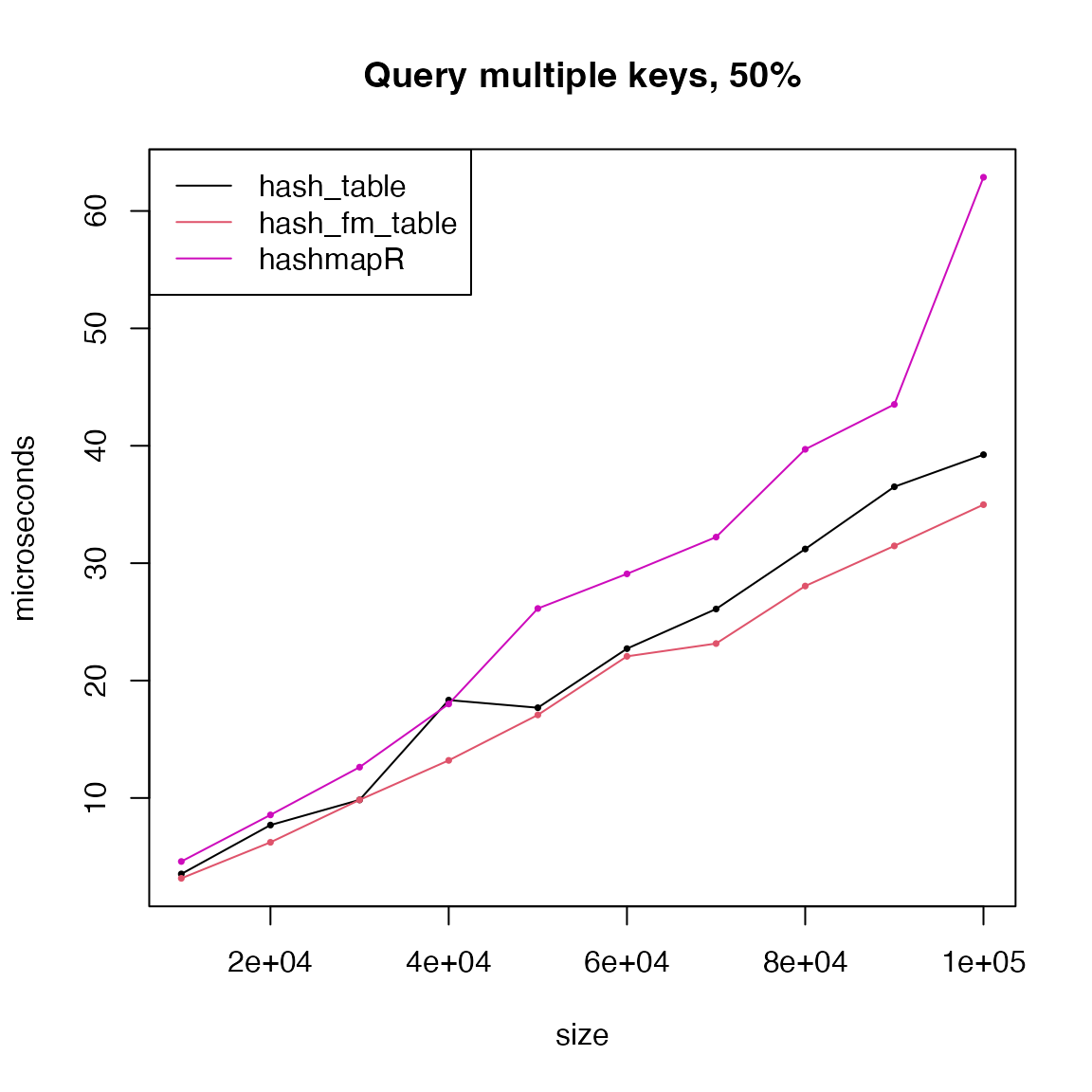

hash_table(), hash_fm_table() and hashmapR only have very small difference.

Insertion

Except hashmapR, all hash table objects created by various methods support [[<- to set a single value. Note hash_fm_table() is not incluced because it does not allow to insert new keys.

Note unique_strings() is based on MD5 hashes of integers, rnorm(1) generates numeric values, so digest(rnorm(1)) generates new keys.

t1 = t3 = t4 = t5 = t6 = t7 = numeric(length(size))
for(i in seq_along(size)) {
    keys = unique_strings(size[i])
    values = seq_along(keys)

    h1 = hash_table(keys = keys, values = values)
    h3 = hash_env_table(keys = keys, values = values)
    
    lt = split(values, keys)
    h4 = list2env(lt, hash = TRUE, parent = emptyenv())

    h5 = hash::hash(keys = keys, values = values)
    
    h6 = hashmapR::hashmap()
    h6$set(split(keys, keys), split(values, keys), vectorize = TRUE)

    h7 = r2r::hashmap()
    h7[keys] = values
    
    t1[i] = bm(h1[[digest(rnorm(1))]] <- 1L)
    t3[i] = bm(h3[[digest(rnorm(1))]] <- 1L)
    t4[i] = bm(h4[[digest(rnorm(1))]] <- 1L)
    t5[i] = bm(h5[[digest(rnorm(1))]] <- 1L)
    t6[i] = bm(h6$set(digest(rnorm(1)), 1L))
    t7[i] = bm(h7[[digest(rnorm(1))]] <- 1L)
}
matplot(size, cbind(t1, t3, t4, t5, t6, t7)/1000, type = "o", 
    lty = 1, col = c(1, 3:7), pch = 16, cex = 0.5, 
    xlab = "size", ylab = "microseconds", main = "Insert a single key")
legend("topleft", lty = 1, col = c(1, 3:7), 
    legend = c("hash_table", "hash_env_table", "list2env", "hash", "hashmapR", "r2r"))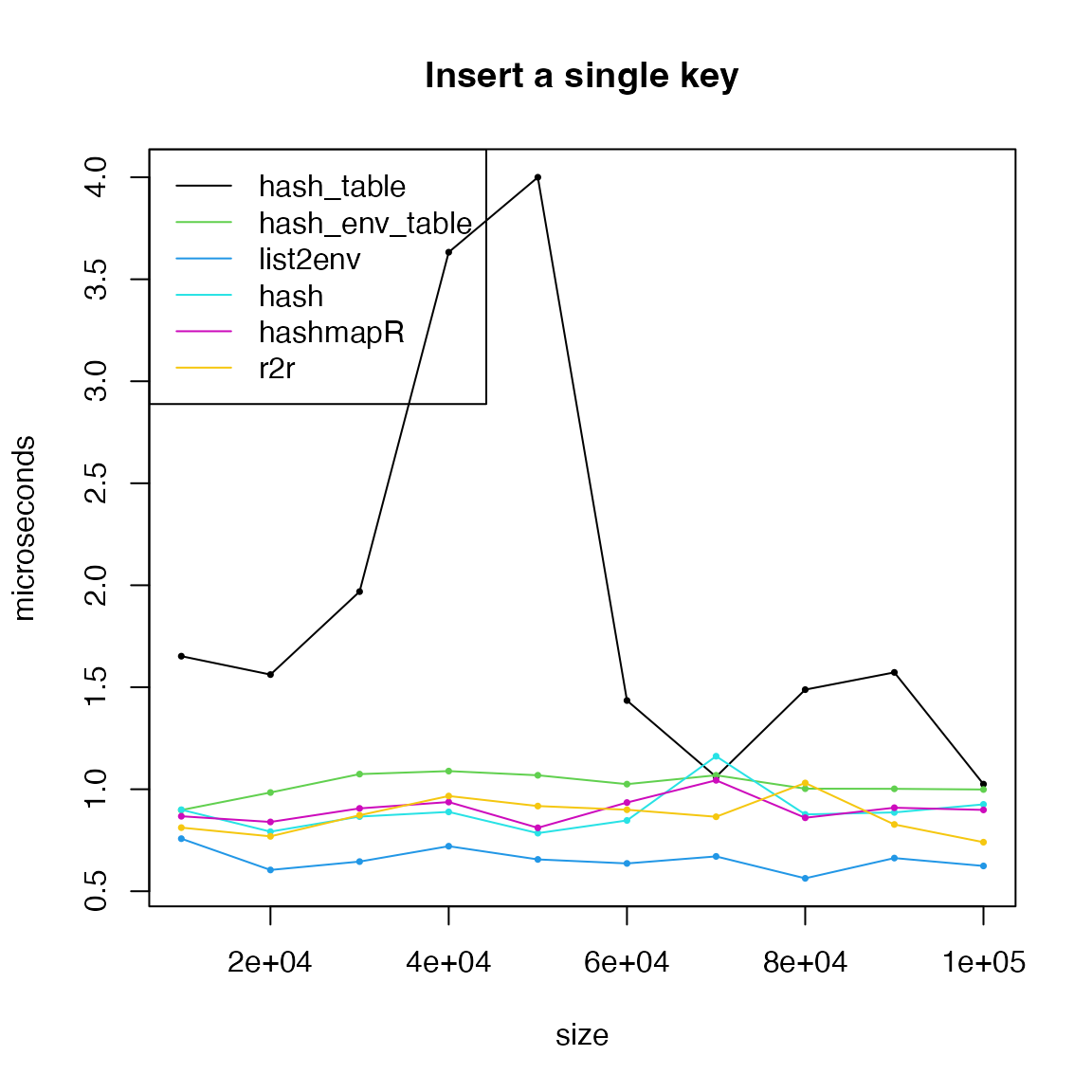

Deletion

Difference methods have different interfaces to delete key-value pairs. hash_fm_table() is not incluced because it does not allow to delete keys.

t1 = t3 = t4 = t5 = t6 = t7 = numeric(length(size))
for(i in seq_along(size)) {
    keys = unique_strings(size[i])
    values = seq_along(keys)

    h1 = hash_table(keys = keys, values = values)
    h3 = hash_env_table(keys = keys, values = values)
    
    lt = split(values, keys)
    h4 = list2env(lt, hash = TRUE, parent = emptyenv())

    h5 = hash::hash(keys = keys, values = values)
    
    h6 = hashmapR::hashmap()
    h6$set(split(keys, keys), split(values, keys), vectorize = TRUE)

    h7 = r2r::hashmap()
    h7[keys] = values
    
    t1[i] = bm(hash_delete(h1, sample(keys, 1)))
    t3[i] = bm(hash_delete(h3, sample(keys, 1)))
    t4[i] = bm(rm(list = sample(keys, 1), h4))
    t5[i] = bm(hash::delete(sample(keys, 1), h5))
    t6[i] = bm(h6$remove(sample(keys, 1)))
    t7[i] = bm(r2r::delete(h7, sample(keys, 1)))
}
matplot(size, cbind(t1, t3, t4, t5, t6, t7)/1000, type = "o", 
    lty = 1, col = c(1, 3:7), pch = 16, cex = 0.5, 
    xlab = "size", ylab = "microseconds", main = "Delete a single key")
legend("left", lty = 1, col = c(1, 3:7), 
    legend = c("hash_table", "hash_env_table", "list2env", "hash", "hashmapR", "r2r"))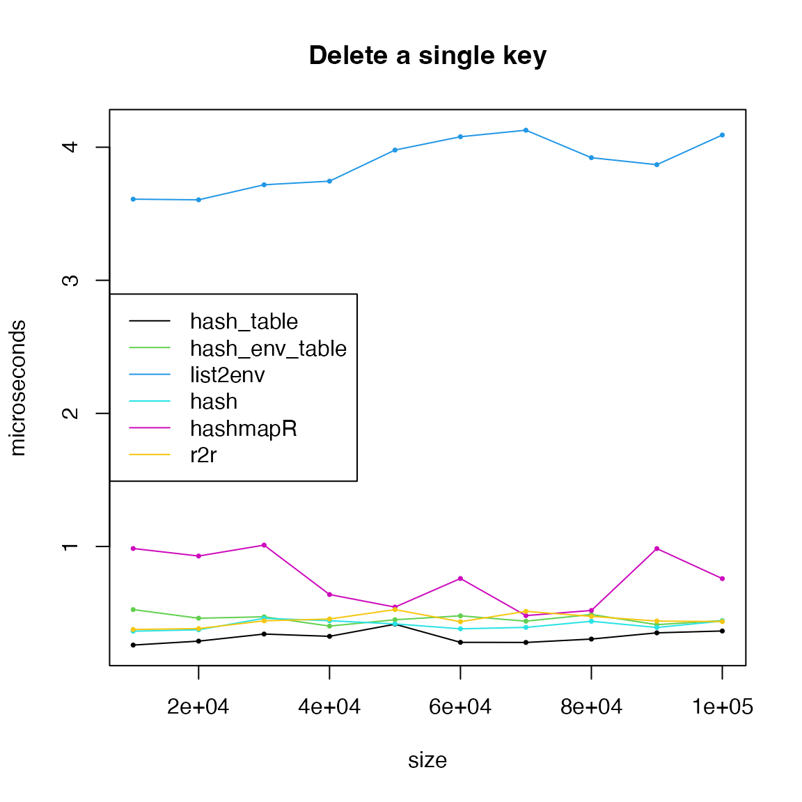

list2env() performs obviously bad. Note for environment, we did not use h4[[key]] = NULL because it just assign NULL to key but the key still exists.

Compare to match-family functions

People may think named vectors (including lists) behave like hashes.

vec = c("foo" = 1, "bar" = 2)
vec

## foo bar 
##   1   2

vec[["foo"]]

## [1] 1

lt = list("foo" = 1, "bar" = "text")
lt$foo

## [1] 1

Actually they are not. Names are just normal character vectors, but attached to the object as an attributes.

attributes(vec)

## $names
## [1] "foo" "bar"

attributes(lt)

## $names
## [1] "foo" "bar"

So using names as indices basically does matching in the “names” attributes.

There are following match-family functions:

pmatch(), used in names(), $, [[, [,
match(), used in %in%, intersect(), unique(), duplicated(),
fastmatch, a faster version of match(), synonyms functions are fmatch() and %fin%,
data.table::chmatch(), also a faster version of match(), synonyms functions are chmatch() and %chin%.

pmatch() means partial matching. It matches elements if substrings can be uniquely mapped.

match(), fastmatch and chmatch() do the complete matching. They have the same interface：

function(x, table, ...)

where x is the query vector, i.e. the keys, and table is the data vector, i.e. all keys. First, all of match(), fastmatch and chmatch() internally generate hash tables for fast matching. The difference is match() and chmatch() generate hash tables in every function call, which means, even table is the same, multiple calls to match() or chmatch(), the internal hash table needs to be rebuilt, while fastmatch directly attaches the hash table to table as an internal attribute, so in afterward repeated calls of fastmatch::fmatch(), the hash table can be directly reused.

library(fastmatch)
library(data.table)
t1 = t2 = t3 = t4 = t5 = t6 = t7 = t8 = numeric(length(size))
for(i in seq_along(size)) {
    keys = unique_strings(size[i])
    values = seq_along(keys)

    x = structure(values, names = keys)

    h1 = hash_table(keys = keys, values = values)
    h2 = hash_fm_table(keys = keys, values = values)
    h3 = hash_env_table(keys = keys, values = values)

    t1[i] = bm(h1[[sample(keys, 1)]])
    t2[i] = bm(h2[[sample(keys, 1)]])

    h6 = hashmapR::hashmap()
    h6$set(split(keys, keys), split(values, keys), vectorize = TRUE)
    t6[i] = bm(h6$get(sample(keys, 1)))

    t4[i] = bm(x[[sample(keys, 1)]])
    t5[i] = bm(x[[match(sample(keys, 1), keys)]])
    t7[i] = bm(x[[fmatch(sample(keys, 1), keys)]])
    t8[i] = bm(x[[chmatch(sample(keys, 1), keys)]])
}
matplot(size, cbind(t1, t2, t3, t6, t4, t5, t7, t8)/1000, type = "o", 
    lty = 1, col = c(1:3, 6, 4, 5, 7, 8), pch = 16, cex = 0.5, 
    xlab = "size", ylab = "microseconds", main = "Query a single key, match-family")
legend("topleft", lty = 1, col = c(1:3, 6, 4, 5, 7, 8), 
    legend = c("hash_table", "hash_fm_table", "hash_env_table", "hashmapR", "pmatch/names", "match", "fastmatch", "chmatch"))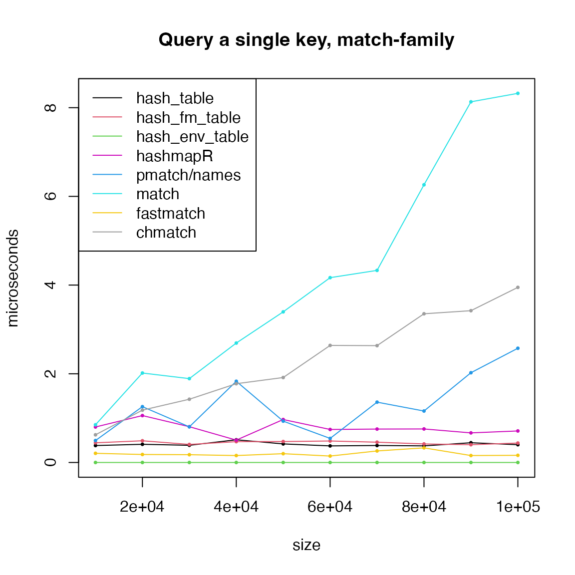

We can see hash-family functions have time complexity of $O(1)$ to the hash table size once the hash table is already created. fastmatch is also fast because the hash table only needs to be calculated once. pmatch(), match() and chmatch() have linear complexity to the size of “the data vector”.

Next query multiple keys with match-family functions.

par(mfrow = c(2, 2))
for(p in c(0.01, 0.1, 0.25, 0.5)) {
    t1 = t2 = t3 = t4 = t5 = t6 = t7 = numeric(length(size))
    for(i in seq_along(size)) {
        keys = unique_strings(size[i])
        values = seq_along(keys)

        x = structure(values, names = keys)

        h1 = hash_table(keys = keys, values = values)
        h2 = hash_fm_table(keys = keys, values = values)
        h3 = hash_env_table(keys = keys, values = values)

        t1[i] = bm(h1[sample(keys, round(p*size[i]))])
        t2[i] = bm(h2[sample(keys, round(p*size[i]))])
        t3[i] = bm(h3[sample(keys, round(p*size[i]))])

        h6 = hashmapR::hashmap()
        h6$set(split(keys, keys), split(values, keys), vectorize = TRUE)
        t6[i] = bm(h6$get(sample(keys, round(p*size[i]))))
            
        t4[i] = bm(x[sample(keys, round(p*size[i]))])
        t5[i] = bm(x[match(sample(keys, round(p*size[i])), keys)])
        t7[i] = bm(x[fmatch(sample(keys, round(p*size[i])), keys)])
        t8[i] = bm(x[chmatch(sample(keys, round(p*size[i])), keys)])
    }
    matplot(size, cbind(t1, t2, t3, t6, t4, t5, t7, t8)/1000, type = "o", 
        lty = 1, col = c(1:3, 6, 4, 5, 7, 8), pch = 16, cex = 0.5, 
        xlab = "size", ylab = "microseconds", main = paste0("Query multiple keys, match-family, ", p*100, "%"))
    legend("topleft", lty = 1, col = c(1:3, 6, 4, 5, 7, 8), 
        legend = c("hash_table", "hash_fm_table", "hash_env_table", "hashmapR", "pmatch/names", "match", "fastmatch", "chmatch"))
}

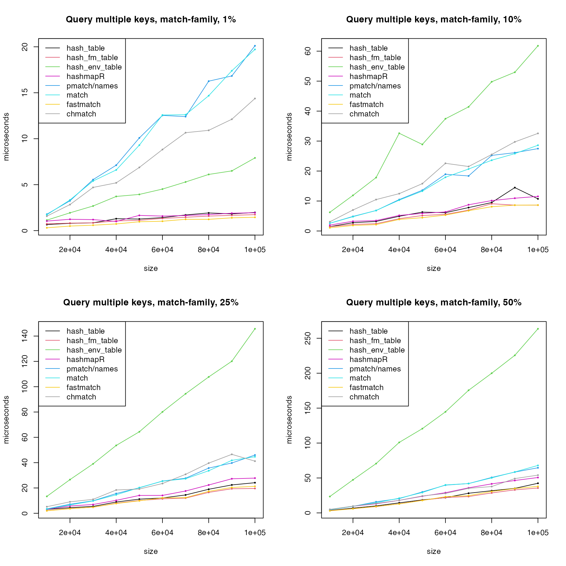
Now the match-family functions have good performance when querying multiple keys. As has been explained, for multiple calls, match-family functions performs bad because the internal hash tables have to be rebuilt, but for multiple key queries in a single call, keys can be directly queried from the internal hash table.

Remove hash_env_table() and remake the last plot.

matplot(size, cbind(t1, t2, t6, t4, t5, t7, t8)/1000, type = "o", 
    lty = 1, col = c(1:2, 6, 4, 5, 7, 8), pch = 16, cex = 0.5, 
    xlab = "size", ylab = "microseconds", main = paste0("Query multiple keys, match-family, ", p*100, "%"))
legend("topleft", lty = 1, col = c(1:2, 6, 4, 5, 7, 8), 
    legend = c("hash_table", "hash_fm_table", "hashmapR", "pmatch/names", "match", "fastmatch", "chmatch"))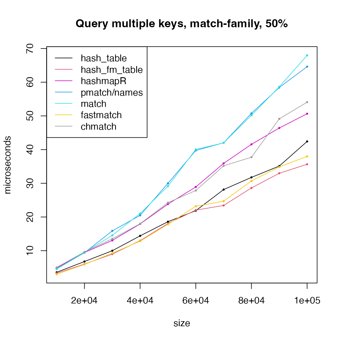

Hash set

Hash set is basically very similar as hash table. The only difference is for hash table, there are values associated with keys, while for hash set, there are only keys.

We first test querying a single key, which is to test whether the key exists in the hash set.

t1 = t2 = t3 = t4 = t5 = t6 = t7 = numeric(length(size))
for(i in seq_along(size)) {
    keys = unique_strings(size[i])

    h1 = hash_set(keys)
    h2 = hash_fm_set(keys)
    h3 = hash_env_set(keys)
    h7 = r2r::hashset(keys)

    t1[i] = bm(h1[[sample(keys, 1)]])
    t2[i] = bm(h2[[sample(keys, 1)]])
    t3[i] = bm(h3[[sample(keys, 1)]])
    t7[i] = bm(h7[[sample(keys, 1)]])

    t4[i] = bm(match(sample(keys, 1), keys))
    t5[i] = bm(fmatch(sample(keys, 1), keys))
    t6[i] = bm(chmatch(sample(keys, 1), keys))
}
matplot(size, cbind(t1, t2, t3, t7, t4, t5, t6)/1000, type = "o", 
    lty = 1, col = c(1:3, 7, 4:6), pch = 16, cex = 0.5, 
    xlab = "size", ylab = "microseconds", main = "Query a single key")
legend("topleft", lty = 1, col = c(1:3, 7, 4:6), 
    legend = c("hash_set", "hash_fm_set", "hash_env_set", "r2r", "match", "fastmatch", "chmatch"))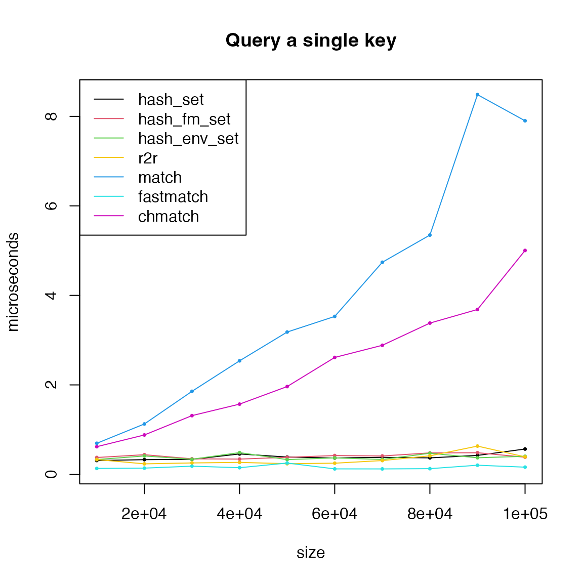

We remove match() and chmatch() and remake the last plot.

matplot(size, cbind(t1, t2, t3, t7, t5)/1000, type = "o", 
    lty = 1, col = c(1:3, 7, 5), pch = 16, cex = 0.5, 
    xlab = "size", ylab = "microseconds", main = "Query a single key")
legend("topleft", lty = 1, col = c(1:3, 7, 5), 
    legend = c("hash_set", "hash_fm_set", "hash_env_set", "r2r", "fastmatch"))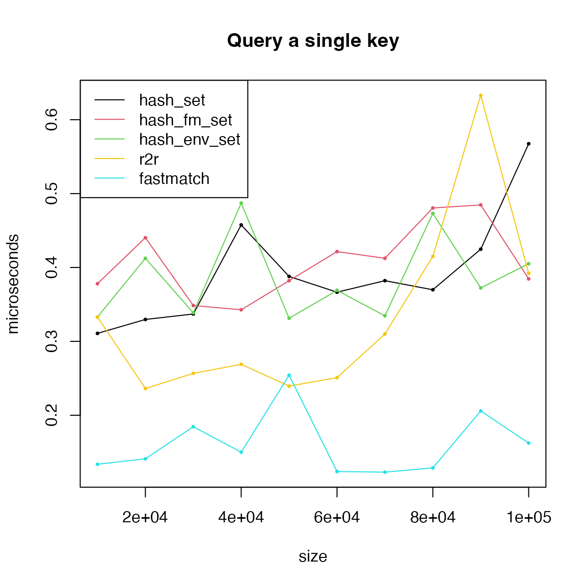

Next query multiple keys.

par(mfrow = c(2, 2))
for(p in c(0.01, 0.1, 0.25, 0.5)) {
    t1 = t2 = t3 = t4 = t5 = t6 = t7 = numeric(length(size))
    for(i in seq_along(size)) {
        keys = unique_strings(size[i])

        h1 = hash_set(keys)
        h2 = hash_fm_set(keys)
        h3 = hash_env_set(keys)
        h7 = r2r::hashset(keys)

        t1[i] = bm(h1[sample(keys, round(p*size[i]))])
        t2[i] = bm(h2[sample(keys, round(p*size[i]))])
        t3[i] = bm(h3[sample(keys, round(p*size[i]))])
        t7[i] = bm(h7[sample(keys, round(p*size[i]))])

        t4[i] = bm(match(sample(keys, round(p*size[i])), keys))
        t5[i] = bm(fmatch(sample(keys, round(p*size[i])), keys))
        t6[i] = bm(chmatch(sample(keys, round(p*size[i])), keys))
    }
    matplot(size, cbind(t1, t2, t3, t7, t4, t5, t6)/1000, type = "o", 
        lty = 1, col = c(1:3, 7, 4:5), pch = 16, cex = 0.5, 
        xlab = "size", ylab = "microseconds", main = paste0("Query multiple keys, ", p*100, "%"))
    legend("topleft", lty = 1, col = c(1:3, 7, 4:6), 
        legend = c("hash_set", "hash_fm_set", "hash_env_set", "r2r", "match", "fastmatch", "chmatch"))
}

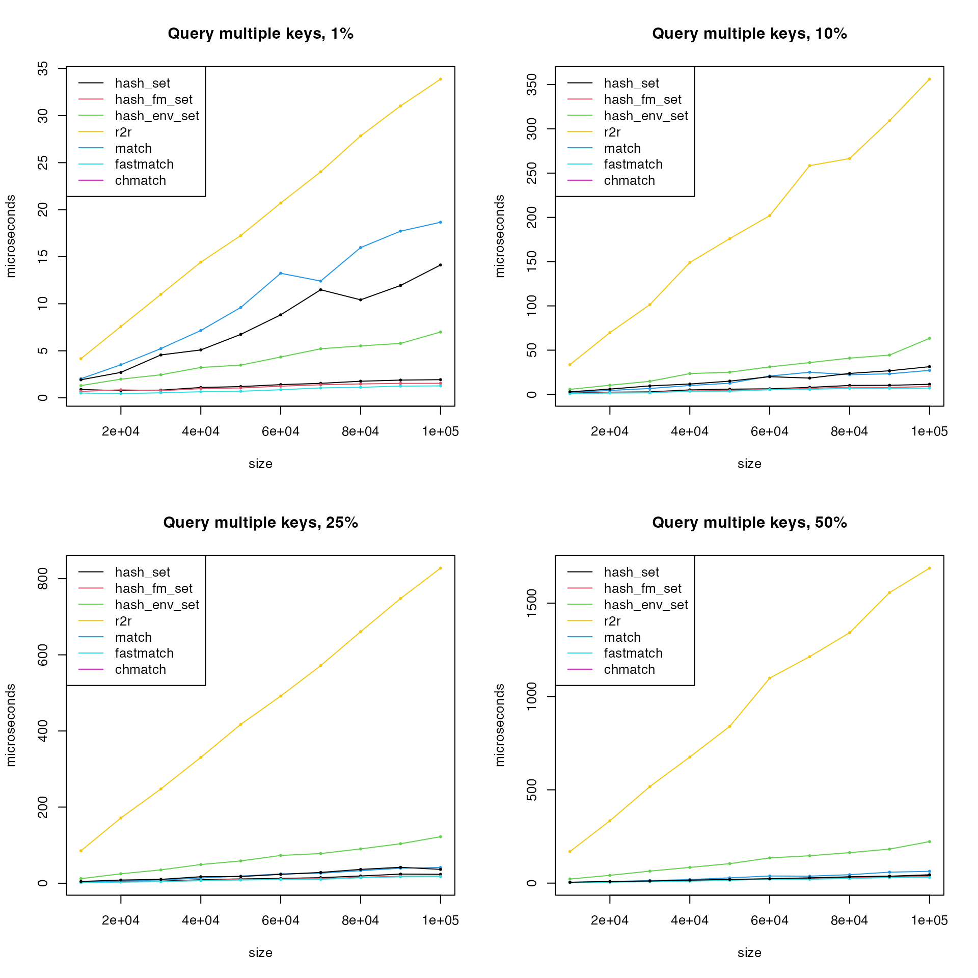
Obviously r2r has very bad performance when querying multiple keys. Remove r2r also hash_env_set() and remake the last plot.

matplot(size, cbind(t1, t2, t4, t5, t6)/1000, type = "o", 
    lty = 1, col = c(1:2, 4:6), pch = 16, cex = 0.5, 
    xlab = "size", ylab = "microseconds", main = paste0("Query multiple keys, ", p*100, "%"))
legend("topleft", lty = 1, col = c(1:2, 4:6), 
    legend = c("hash_set", "hash_fm_set", "match", "fastmatch", "chmatch"))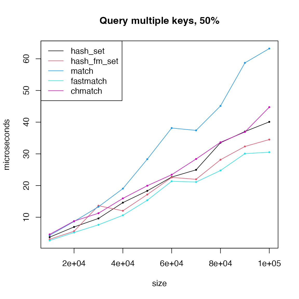

Compare hash tables and hash sets

In hashtable, hash tables and hash sets are implements similarly in the three implementations.

t1 = t2 = t3 = t4 = t5 = t6 = numeric(length(size))
for(i in seq_along(size)) {
    keys = unique_strings(size[i])
    values = seq_len(size[i])

    h1 = hash_table(keys = keys, values = values)
    h2 = hash_fm_table(keys = keys, values = values)
    h3 = hash_env_table(keys = keys, values = values)

    h4 = hash_set(keys = keys)
    h5 = hash_fm_set(keys = keys)
    h6 = hash_env_set(keys = keys)
    
    p = 0.1
    t1[i] = bm(h1[sample(keys, round(p*size[i]))])
    t2[i] = bm(h2[sample(keys, round(p*size[i]))])
    t3[i] = bm(h3[sample(keys, round(p*size[i]))])
    t4[i] = bm(h4[sample(keys, round(p*size[i]))])
    t5[i] = bm(h5[sample(keys, round(p*size[i]))])
    t6[i] = bm(h6[sample(keys, round(p*size[i]))])
}
matplot(size, cbind(t1, t2, t3, t4, t5, t6)/1000, type = "o", 
    lty = c(1, 1, 1, 2, 2, 2), col = c(1, 2, 3, 1, 2, 3), pch = 16, cex = 0.5, 
    xlab = "size", ylab = "microseconds", main = "Query multiple keys")
legend("topleft", lty = c(1, 1, 1, 2, 2, 2), col = c(1, 2, 3, 1, 2, 3), 
    legend = c("hash_table", "hash_fm_table", "hash_env_table", "hash_set", "hash_fm_set", "hash_env_set"))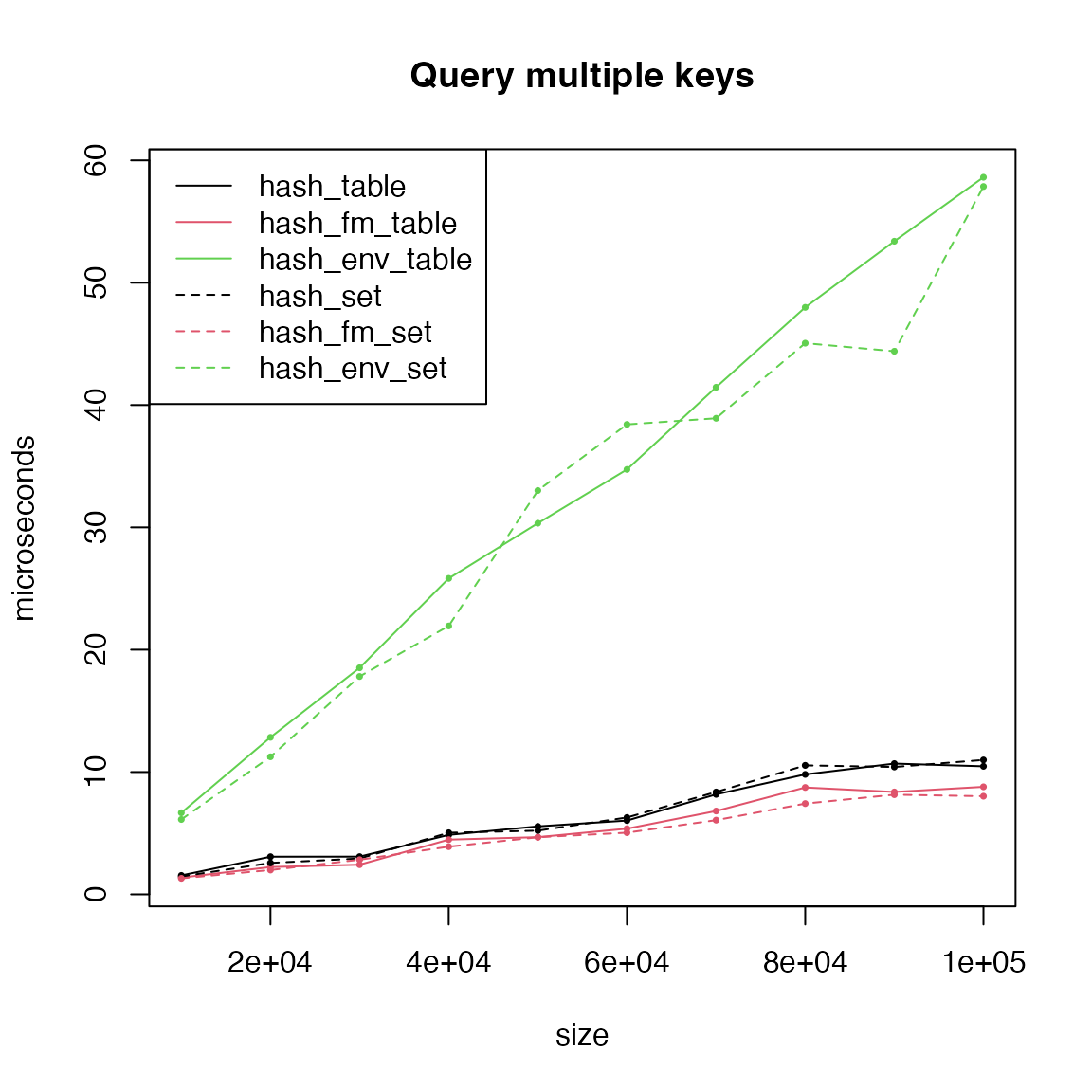

Summarize

For creating hash tables, hashtable is fast.

For querying single keys, all hash-functions are fast, but the runtime of pmatch(), match() and chmatch() increases linearly to the size of the data.

For querying multiple keys, hash_fm_set() and fmatch() is the fastest. If hash tables are changable, then hash_table() and hashmapR can be considered as replacement.

For inserting new keys, all hash-functions are similar.

For deleting keys, list2env() (which uses rm()) is relatively slow. Other functions are similar.

sessionInfo()

## R version 4.6.0 (2026-04-24)
## Platform: aarch64-apple-darwin23
## Running under: macOS Tahoe 26.5.1
## 
## Matrix products: default
## BLAS:   /Library/Frameworks/R.framework/Versions/4.6/Resources/lib/libRblas.0.dylib 
## LAPACK: /Library/Frameworks/R.framework/Versions/4.6/Resources/lib/libRlapack.dylib;  LAPACK version 3.12.1
## 
## locale:
## [1] en_GB.UTF-8/en_GB.UTF-8/en_GB.UTF-8/C/en_GB.UTF-8/en_GB.UTF-8
## 
## time zone: Asia/Shanghai
## tzcode source: internal
## 
## attached base packages:
## [1] stats     graphics  grDevices utils     datasets  methods   base     
## 
## other attached packages:
## [1] data.table_1.18.4    fastmatch_1.1-8      digest_0.6.39       
## [4] microbenchmark_1.5.0 hashtable_1.0.0      knitr_1.51          
## 
## loaded via a namespace (and not attached):
##  [1] cli_3.6.6         rlang_1.2.0       xfun_0.59         otel_0.2.0       
##  [5] textshaping_1.0.5 jsonlite_2.0.0    hash_2.2.6.4      htmltools_0.5.9  
##  [9] ragg_1.5.2        sass_0.4.10       rmarkdown_2.31    evaluate_1.0.5   
## [13] jquerylib_0.1.4   fastmap_1.2.0     yaml_2.3.12       lifecycle_1.0.5  
## [17] hashmapR_1.0.1    compiler_4.6.0    fs_2.1.0          htmlwidgets_1.6.4
## [21] Rcpp_1.1.1-1.1    systemfonts_1.3.2 R6_2.6.1          bslib_0.11.0     
## [25] tools_4.6.0       r2r_0.1.2         pkgdown_2.2.0     cachem_1.1.0     
## [29] desc_1.4.3

Zuguang Gu ( guzuguang@suat-sz.edu.cn )

2026-07-09