Visualize Categorical Signals
Zuguang Gu ( z.gu@dkfz.de )
2024-02-27
Source:vignettes/visualize_categorical_signals.Rmd
visualize_categorical_signals.RmdNormally genomic signals are represented as numeric (e.g. methylation from WGBS or histone modification intensity from ChIP-seq) or binary values (e.g. existance of CpG islands in a given position), however, genomic signals sometimes can also be represented as categorical or discrete values (mostly stored as characters). A very typical example is chromatin states segmentation by ChromHMM. ChromHMM basically assigns a chromatin state (e.g. active transcription state or repressive transcription state) to a given window in the genome and the assignment of states in different windows are always mutually exclusive (which means one window can only have one state). In this vignette, We will demonstrate how to visualize the enrichment of various chromatin states around certain genomic targets and how to integerate with other epigenomic signals.
General examples
In following example, we use Roadmap dataset as the example dataset. First we show basic usages with using one sample (sample id: E003, embryonic stem cell, H1 cell line).
Load packages:
The chromatin state segmentation is trained and applied from five histone modifications. Following file in use is from http://egg2.wustl.edu/roadmap/data/byFileType/chromhmmSegmentations/ChmmModels/coreMarks/jointModel/final/E003_15_coreMarks_mnemonics.bed.gz.
We convert to a GRanges object.
states_bed = fread("zcat ~/EnrichedHeatmap_test/E003_15_coreMarks_mnemonics.bed.gz")
states = GRanges(seqnames = states_bed[[1]],
  ranges = IRanges(states_bed[[2]] + 1, states_bed[[3]]),
  states = states_bed[[4]])
unique(states_bed[[4]])
## [1] "15_Quies" "9_Het" "14_ReprPCWk" "13_ReprPC" "10_TssBiv" "7_Enh"
## [7] "1_TssA" "11_BivFlnk" "2_TssAFlnk" "5_TxWk" "4_Tx" "8_ZNF/Rpts"
## [13] "6_EnhG" "12_EnhBiv" "3_TxFlnk"In the 15 states, there are some states which are similar to each other such as 1_TssA (active TSS) and 2_TssAFlnk (flanking active TSS). To reduce the complexity of the analysis, we merge some of the similar states.
map = c(
  "1_TssA"      = "TssActive",
  "2_TssAFlnk"  = "TssActive",
  "3_TxFlnk"    = "Transcript",
  "4_Tx"        = "Transcript",
  "5_TxWk"      = "Transcript",
  "6_EnhG"      = "Enhancer",
  "7_Enh"       = "Enhancer",
  "8_ZNF/Rpts"  = "Heterochromatin",
  "9_Het"       = "Heterochromatin",
  "10_TssBiv"   = "TssBivalent",
  "11_BivFlnk"  = "TssBivalent",
  "12_EnhBiv"   = "Enhancer",
  "13_ReprPC"   = "Repressive",
  "14_ReprPCWk" = "Repressive",
  "15_Quies"    = "Quiescent"
)
states$states_simplified = map[states$states]
Also we set the colors for the 7 merged states.
states_col = c(
  "TssActive"       = "Red",
  "Transcript"      = "Green",
  "Enhancer"        = "Yellow",
  "Heterochromatin" = "PaleTurquoise",
  "TssBivalent"     = "Orange",
  "Repressive"      = "Grey",
  "Quiescent"       = "black"
)
states_name = names(states_col)
n_states = length(states_col)
In following, we demonstrate how to normalize the chromatin states to TSS. First we load the transcriptome and extract TSS regions. The transcriptome annotation is from http://egg2.wustl.edu/roadmap/data/byDataType/rna/annotations/gen10.long.gtf.gz and we only use protein coding genes. The database file (the sqlite file) for transcriptome was generated by GenomicFeatures package (the makeTxDbFromGFF() function).
library(GenomicFeatures)
txdb = loadDb("~/EnrichedHeatmap_test/gencode10_protein_coding_txdb.sqlite")

g = genes(txdb)
tss = promoters(g, upstream = 0, downstream = 1)
To reduce the running time, here we only use chromosome 1. Normalizing categorical signals is basically as same as numeric signals. Here we only need to specify the column name for the categorical signals.
tss_chr1 = tss[seqnames(tss) == "chr1"]
# column "states_simplified" is in character mode
mat_states = normalizeToMatrix(states, tss_chr1, value_column = "states_simplified")
mat_states
## Normalize states to tss_chr1:
## Upstream 5000 bp (50 windows)
## Downstream 5000 bp (50 windows)
## Include target regions (width = 1)
## 2065 target regions
## signal is categorical (7 levels)In the last line of the message, it clarifies it is categorical signals with 7 levels.
The implementation of normalizing categorical signals is actually very simple. Internally, n_states normalized matrices are generated where each one corresponds to one chromatin state and the value in each window is the fraction how much the window is overlapped to the state (with w0 or weighted mean mode). Since the i^th row and the j^th column in all matrices correspond to a same window to a same target (here the TSS), if there are multiple states overlap to this same window, when summarizing from all states, the state with largest overlap fraction is assigned to this window.
Since the normalizeToMatrix() is called n_states times internally, it will be a little bit slow to normalize to categorical signals.
There are some special visualizations designed for categorical signals where each state is summarized and visualized separatedly in the top annotation. Here states_col must be a named vector where the names should correspond to the levels of the categorical signals.
EnrichedHeatmap(mat_states, name = "states", col = states_col)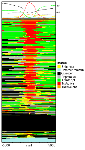
plot of chunk categorical_default
You might feel the row ordering is a little bit in a mess. Although the signals are categorical, internally, there are coded as integer numbers. Just similar as how factor in R is stored, each categorical level corresponds to an integer number. If the signal column is simply a character vector, the assignment of integers are based on the natural ordering of this character vector. Thus the numeric coding for signals in states object is:
data.frame(states = unique(states$states_simplified), value = 1:7)## states value
## 1 Quiescent 1
## 2 Heterochromatin 2
## 3 Repressive 3
## 4 TssBivalent 4
## 5 Enhancer 5
## 6 TssActive 6
## 7 Transcript 7Zero is assigned to a window if none of the states overlap to it and it is drawn with white.
The numeric coding can be controlled by setting the signals as a factor variable and the level order of the factor controls the corresponding coding. In following code, we convert states_simplified as a factor with specifying the level order.
states$states_simplified = factor(states$states_simplified, levels = states_name)
data.frame(states = levels(states$states_simplified), value = 1:7)
## states value
## 1 TssActive 1
## 2 Transcript 2
## 3 Enhancer 3
## 4 Heterochromatin 4
## 5 TssBivalent 5
## 6 Repressive 6
## 7 Quiescent 7Note here the order of states_name also reflects the closeness of different states. With the order defined above, TssActive is closer to Transcript and Repressive is closer to Quiescent.
In following left plot, the TSS with active states now are far from the TSS with repressive states. In the right plot we change the level of states_simplified and you can compare to the left one.
mat_states = normalizeToMatrix(states, tss_chr1, value_column = "states_simplified")
EnrichedHeatmap(mat_states, name = "states", col = states_col)
# shuffle levels for states_simplified
states$states_simplified = factor(states$states_simplified,
  levels = states_name[c(1, 6, 2, 7, 4, 3, 5)])
mat_states = normalizeToMatrix(states, tss_chr1, value_column = "states_simplified")
EnrichedHeatmap(mat_states, name = "states", col = states_col,
  row_title = "states_name[c(1, 6, 2, 7, 4, 3, 5)]")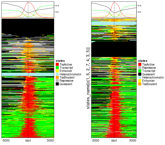
plot of chunk unnamed-chunk-10
We suggest to apply hierarchical clustering to reorder rows. Here the numeric coding is espeically important because it affects the calculation of distance between rows.
# we change the level back
states$states_simplified = factor(states$states_simplified, levels = states_name)
mat_states = normalizeToMatrix(states, tss_chr1, value_column = "states_simplified")
EnrichedHeatmap(mat_states, name = "states", col = states_col, cluster_rows = TRUE)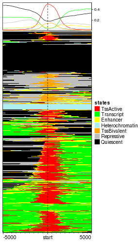
plot of chunk categorical_clustered
Since the normalized matrix is numeric, k-means clustering can also be applied.
EnrichedHeatmap(mat_states, name = "states", col = states_col, cluster_rows = TRUE, row_km = 2)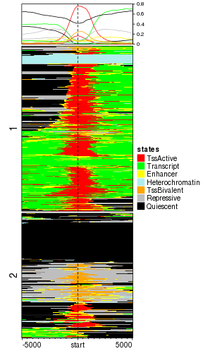
plot of chunk categorical_kmeans
After closely looking at the heatmap, we found the TSS states are consistently enriched around TSS while in the flanking regions, the states are a little bit diverse. Actually this suggests that in order to enhance the pattern of the TSS-related states, we can apply k-means clustering only for the states near TSS regions.
In following we only cluster the sub-matrix which is upstrean and downstream 1kb of TSS (The default extension of TSS is 5kb upstream and downstream, the number of columns in the normalized matrix is 100, thus from 40^th column to 60^th column are the states in 1kb upstream and downstream of TSS).
Of couse we need to calculate this partitioning in advance.
split = kmeans(mat_states[, 40:60], centers = 2)$cluster
EnrichedHeatmap(mat_states, name = "states", col = states_col, cluster_rows = TRUE,
  row_split = split)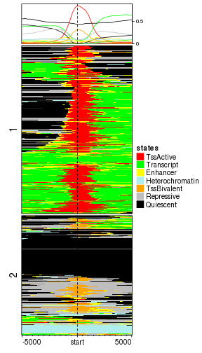
plot of chunk categorical_partial_kmeans
Now it is quite nice to see genes with active TSS are all clustered in cluster 2 while in cluster 1, genes are either have no function or have bivalent TSS function.
Similarly, we can visualize how the chromatin states enriched at gene bodies. Since the gene bodies have unequal widths, we add an additional point plot to show the width of genes.
g_chr1 = g[seqnames(g) == "chr1"]
mat_states_2 = normalizeToMatrix(states, g_chr1, value_column = "states_simplified")
EnrichedHeatmap(mat_states_2, name = "states", col = states_col, cluster_rows = TRUE) +
rowAnnotation(gene_len = anno_points(log10(width(g_chr1) + 1), size = unit(1, "mm"),
  axis = TRUE, axis_param = list(at = c(2, 3, 4, 5, 6),
    labels = c("100bp", "1kb", "10kb", "100kb", "1mb")),
  width = unit(4, "cm")))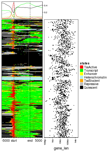
plot of chunk categorical_gene_body
Next we add methylation around TSS as well as expression for the corresponding genes. Expression data is from http://egg2.wustl.edu/roadmap/data/byDataType/rna/expression/57epigenomes.RPKM.pc.gz and methylation data is from http://egg2.wustl.edu/roadmap/data/byDataType/dnamethylation/WGBS/FractionalMethylation.tar.gz
In following, the raw methylation data has been smoothed by bsseq package. The rds file was generated by the old version of bsseq package that is why we used a strange way to extract the positions of CpG sites as well as smoothed methylation data which can be replaced by using granges() and getMeth() functions if the smoothing is applied with newest version of bsseq package.
expr = read.table("~/EnrichedHeatmap_test/57epigenomes.RPKM.pc.gz", row.names = 1, header = TRUE)
expr = as.matrix(expr)
obj = readRDS("~/EnrichedHeatmap_test/chr1_roadmap_merged_bsseq.rds")
meth = obj@rowData
meth_mat = obj@trans(obj@assays$data$coef)
mcols(meth) = meth_mat
We take the genes which exist both in tss_chr1 and expr.
names(tss_chr1) = gsub("\\.\\d+$", "", names(tss_chr1))
cn = intersect(names(tss_chr1), rownames(expr))
tss_chr1 = tss_chr1[cn]
expr = expr[cn, ]
We normalize chromatin states as well methylation to TSS on chromosome 1.
mat_states = normalizeToMatrix(states, tss_chr1, value_column = "states_simplified")
mat_meth = normalizeToMatrix(meth, tss_chr1, value_column = "E003", mean_mode = "absolute",
  smooth = TRUE)
Similarly, k-means is applied on chromatin states 1kb upstream and downstream of TSS. Note since the rows are split into two sub-cluster, we add anno_summary() to the expression matrix to show the distribution of expression in the two sub-clusters.
split = kmeans(mat_states[, 40:60], centers = 2)$cluster
meth_col_fun = colorRamp2(c(0, 0.5, 1), c("blue", "white", "red"))
ht_list = EnrichedHeatmap(mat_states, name = "states", col = states_col, cluster_rows = TRUE,
  row_split = split,
  top_annotation = HeatmapAnnotation(enrich = anno_enriched(gp = gpar(lty = 1:2)))) +
EnrichedHeatmap(mat_meth, name = "meth", col = meth_col_fun,
  top_annotation = HeatmapAnnotation(enrich = anno_enriched(gp = gpar(lty = 1:2)))) +
Heatmap(log2(expr[names(tss_chr1), "E003"] + 1), name = "expr",
  show_row_names = FALSE, width = unit(1, "cm"),
  top_annotation = HeatmapAnnotation(summary = anno_summary(gp = gpar(lty = 1:2),
    outline = FALSE, axis_param = list(side = "right"))))
draw(ht_list, ht_gap = unit(8, "mm"))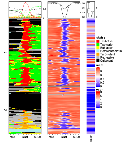
plot of chunk categorical_with_meth
With corresponding to more epigenomic signals, we can see promoters with active TSS states are always associated with low methylation and high gene expression while promoters annotated as bivalent states or repressed are generally more lowly expressed.
Bivalent TSS
It is believed that in embryonic stem cell, there are a huge number of genes showing bivalency states on promoters. They are called bivalent states because both H3K4me3 which is a histone mark for active transcription and H3K27me3 which is for repressive transcription exist. The loss/gain of active histone mark or repressive histone mark which transite into mature cells is essential for tissue development and differentiation.
To demonstate this, we anlaysis such transitions for one mature tissue (lung tissue, roadmap sample id: E096).
states_bed = fread("zcat ~/EnrichedHeatmap_test/E096_15_coreMarks_mnemonics.bed.gz")
states_lung = GRanges(seqnames = states_bed[[1]], ranges = IRanges(states_bed[[2]] + 1, states_bed[[3]]),
  states = states_bed[[4]])
states_lung$states_simplified = factor(map[states_lung$states], levels = states_name)
ChromHMM is performed with 200bp window, thus we split whole genome by 200bp window and assign corresponding states to each window, both for ESC and lung.
window = makeWindows(states, w = 200)
mtch = as.matrix(findOverlaps(window, states))
window$ESC_states = states$states_simplified[mtch[, 2]]
mtch = as.matrix(findOverlaps(window, states_lung))
window$lung_states = states_lung$states_simplified[mtch[, 2]]
We only use the windows which are annotated with TssBivalent state either in ESC or in lung.
window = window[window$ESC_states == "TssBivalent" | window$lung_states == "TssBivalent"]We first make a Chord diagram to show how the transsition happens.
transition_mat = table(mcols(window)[, c("ESC_states", "lung_states")]) * 200
class(transition_mat) = "matrix"
transition_mat = transition_mat[states_name, states_name]
transition_mat
## lung_states
## ESC_states TssActive Transcript Enhancer Heterochromatin TssBivalent Repressive Quiescent
## TssActive 0 0 0 0 136200 0 0
## Transcript 0 0 0 0 8200 0 0
## Enhancer 0 0 0 0 38800 0 0
## Heterochromatin 0 0 0 0 55800 0 0
## TssBivalent 4485600 665400 3711800 653000 406000 1799200 766200
## Repressive 0 0 0 0 24600 0 0
## Quiescent 0 0 0 0 23800 0 0The values in the transition matrix mean how many base pairs change from one chromatin state to the other state.
Rows and columns are from different cells, we add prefix to row and column names.
rownames(transition_mat) = paste0("ESC_", rownames(transition_mat))
colnames(transition_mat) = paste0("lung_", colnames(transition_mat))
Now we make the Chord diagram.
grid.col = c(states_col, states_col)
names(grid.col) = c(rownames(transition_mat), colnames(transition_mat))
chordDiagram(transition_mat, grid.col = grid.col, annotationTrack = c("grid", "axis"),
  directional = TRUE, gap.degree = 5)
circos.clear()
text(0.5, -1, "ESC")
text(0.5, 1, "lung")
legend("left", pch = 15, col = states_col, legend = names(states_col))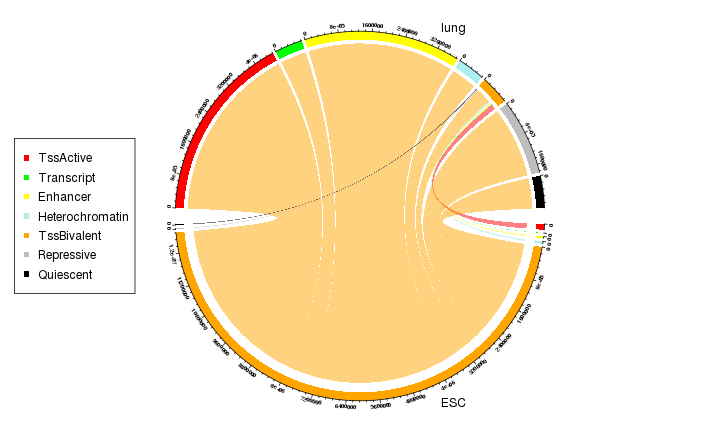
plot of chunk tssbiv_chord_diagram
As we can see from the Chord diagram, a lot of regions with bivalent TSS states (orange track at bottom) have been tansite to active (red track on top) or repressive states (grey track on top) in lung.
To get more deep of how the transistion looks like, we can make enriched heatmaps to see the associations between different epigenomic signals.
Since TssBivalent states basically are states for TSS related regions, we only keep genes for which in 1kb upstream and downstream of TSS there must be a window with TssBivalent state. Again, we only use chromosome 1 as demonstration.
mat_bivtss = normalizeToMatrix(states[states$states_simplified == "TssBivalent"], tss_chr1)
l = rowSums(mat_bivtss[, 40:60]) > 0 # 1kb upstream and downstream
tss_biv = tss_chr1[l]
tss_biv
## GRanges object with 443 ranges and 1 metadata column:
## seqnames ranges strand | gene_id
## <Rle> <IRanges> <Rle> | <character>
## ENSG00000000938 chr1 [ 27961788, 27961788] - | ENSG00000000938.8
## ENSG00000006555 chr1 [ 55266940, 55266940] - | ENSG00000006555.6
## ENSG00000007968 chr1 [ 23857712, 23857712] - | ENSG00000007968.6
## ENSG00000008118 chr1 [209757062, 209757062] + | ENSG00000008118.5
## ENSG00000009709 chr1 [ 18957500, 18957500] + | ENSG00000009709.7
## ... ... ... ... . ...
## ENSG00000243749 chr1 [ 35450954, 35450954] - | ENSG00000243749.1
## ENSG00000248485 chr1 [161228517, 161228517] + | ENSG00000248485.1
## ENSG00000249087 chr1 [ 23695711, 23695711] + | ENSG00000249087.3
## ENSG00000251246 chr1 [155036224, 155036224] + | ENSG00000251246.1
## ENSG00000253304 chr1 [ 29450447, 29450447] - | ENSG00000253304.1
## -------
## seqinfo: 25 sequences from an unspecified genome; no seqlengthsWe normalize chromatin states and methylation to tss_biv.
mat_states_ESC = normalizeToMatrix(states, tss_biv, value_column = "states_simplified")
mat_states_lung = normalizeToMatrix(states_lung, tss_biv, value_column = "states_simplified")

mat_meth_ESC = normalizeToMatrix(meth, tss_biv, value_column = "E003", mean_mode = "absolute",
  smooth = TRUE)
mat_meth_lung = normalizeToMatrix(meth, tss_biv, value_column = "E096", mean_mode = "absolute",
  smooth = TRUE)
Normally, methylation changes happen at the border of low methylation region. To enhance the effect of methylation change, we directly visualize the methyaltion difference.
mat_meth_diff = mat_meth_ESC - mat_meth_lung
meth_diff_col_fun = colorRamp2(c(-0.25, 0, 0.25), c("#3794bf", "#FFFFFF", "#df8640"))
Now we construct the heatmap list.
ht_list = EnrichedHeatmap(mat_states_ESC, name = "states_ESC", col = states_col,
  top_annotation = HeatmapAnnotation(enrich = anno_enriched(gp = gpar(lty = 1:2), ylim = c(0, 1))),
  column_title = "States ESC") +
EnrichedHeatmap(mat_states_lung, name = "states_lung", col = states_col,
  top_annotation = HeatmapAnnotation(enrich = anno_enriched(gp = gpar(lty = 1:2), ylim = c(0, 1))),
  show_heatmap_legend = FALSE, column_title = "States lung")

ht_list = ht_list + EnrichedHeatmap(mat_meth_ESC, name = "meth_ESC", col = meth_col_fun,
  top_annotation = HeatmapAnnotation(enrich = anno_enriched(gp = gpar(lty = 1:2), ylim = c(0, 1))),
  column_title = "Meth ESC") +
EnrichedHeatmap(mat_meth_lung, name = "meth_lung", col = meth_col_fun,
  top_annotation = HeatmapAnnotation(enrich = anno_enriched(gp = gpar(lty = 1:2),
    ylim = c(0, 1))),
  show_heatmap_legend = FALSE, column_title = "Meth lung") +
EnrichedHeatmap(mat_meth_diff, name = "meth_diff", col = meth_diff_col_fun,
  top_annotation = HeatmapAnnotation(enrich = anno_enriched(gp = gpar(lty = 1:2,
    pos_col = "#df8640", neg_col = "#3794bf"))),
  column_title = "Meth ESC - lung")
Actually we can discretize the numeric mat_meth_diff. Here we assign hyper to windows with methylation difference larger than 0.2 and hypo to windows with methylation difference less than -0.2. Here discretize() converts a matrix with continuous signals to categorical signals by prividing a list of intervals.
mat_meth_diff_discrete = discretize(mat_meth_diff,
  rule = list(
    "hypo" = c(-Inf, -0.2),
    "hyper" = c(0.2, Inf)
  )
)
mat_meth_diff_discrete
## Normalize to tss_biv:
## Upstream 5000 bp (50 windows)
## Downstream 5000 bp (50 windows)
## Include target regions (width = 1)
## 443 target regions
## signal is categorical (2 levels)We continue to add more heatmaps.
ht_list = ht_list + EnrichedHeatmap(mat_meth_diff_discrete, name = "meth_diff_discrete",
  col = c("hyper" = "#df8640", hypo = "#3794bf"),
  top_annotation = HeatmapAnnotation(enrich = anno_enriched(gp = gpar(lty = 1:2))))
Finally the heatmap for gene expression.
e = log2(expr[names(tss_biv), c("E003", "E096")] + 1)
ht_list = ht_list + Heatmap(e, name = "expr",
  show_row_names = FALSE, width = unit(10, "mm"), cluster_columns = FALSE)
The row ordering for all heatmaps is from hierarchical clustering on the merged matrix from states in ESC and lung, 1kb upstream and downstream of TSS.
row_order = hclust(dist(cbind(mat_states_ESC[, 40:60], mat_states_lung[, 40:60])))$order
split = ifelse(e[, "E096"] > e[, "E003"], "activation", "repression")
draw(ht_list, row_order = row_order, row_split = split)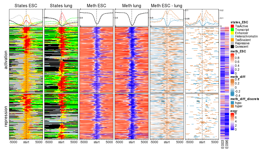
plot of chunk categorical_with_lung
What conclusion can you make from the plot? I can only say the regulation pattern is really complicated there :).
Other examples
There are some other examples where the genomic signals are categorical.
- repeats where different repeat family can be different categories,
- genome segmentation based on methylation. E.g. hign methylated regions (HMRs), partially methylated regions (PMDs), low methylated regions (LMRs), unmethylated regions (UMRs),
- for gene-related regions, genic annotation is also categorical.
Session Info
## R version 3.3.1 (2016-06-21)
## Platform: x86_64-pc-linux-gnu (64-bit)
## Running under: openSUSE 13.1 (Bottle) (x86_64)
##
## locale:
##  [1] LC_CTYPE=en_GB.UTF-8       LC_NUMERIC=C               LC_TIME=en_GB.UTF-8
##  [4] LC_COLLATE=en_GB.UTF-8     LC_MONETARY=en_GB.UTF-8    LC_MESSAGES=en_GB.UTF-8
##  [7] LC_PAPER=en_GB.UTF-8       LC_NAME=C                  LC_ADDRESS=C
## [10] LC_TELEPHONE=C             LC_MEASUREMENT=en_GB.UTF-8 LC_IDENTIFICATION=C
##
## attached base packages:
##  [1] grid      parallel  stats4    stats     graphics  grDevices utils     datasets  methods
## [10] base
##
## other attached packages:
##  [1] GenomicFeatures_1.26.4 AnnotationDbi_1.36.2   Biobase_2.34.0         circlize_0.4.5
##  [5] EnrichedHeatmap_1.13.1 ComplexHeatmap_1.99.0  data.table_1.10.4      GenomicRanges_1.26.4
##  [9] GenomeInfoDb_1.10.3    IRanges_2.8.2          S4Vectors_0.12.2       BiocGenerics_0.20.0
## [13] markdown_0.8           knitr_1.20             colorout_1.2-0
##
## loaded via a namespace (and not attached):
##  [1] Rcpp_0.12.18               highr_0.7                  RColorBrewer_1.1-2
##  [4] XVector_0.14.1             bitops_1.0-6               tools_3.3.1
##  [7] zlibbioc_1.20.0            biomaRt_2.30.0             evaluate_0.11
## [10] RSQLite_1.0.0              lattice_0.20-34            png_0.1-7
## [13] Matrix_1.2-7.1             DBI_1.0.0                  rtracklayer_1.34.2
## [16] stringr_1.3.1              Biostrings_2.42.1          GlobalOptions_0.1.0
## [19] locfit_1.5-9.1             GetoptLong_0.1.7           BiocParallel_1.8.2
## [22] XML_3.98-1.16              magrittr_1.5               GenomicAlignments_1.10.1
## [25] Rsamtools_1.26.2           matrixStats_0.54.0         SummarizedExperiment_1.4.0
## [28] shape_1.4.4                colorspace_1.3-2           stringi_1.2.4
## [31] RCurl_1.95-4.8             rjson_0.2.20