Word cloud as heatmap annotation

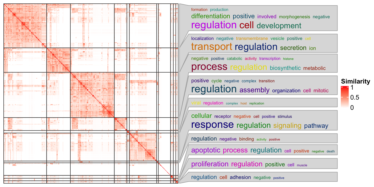
I am recently developing a new package simplifyEnrichment which clusters GO terms into clusters and visualizes the summaries of GO terms in each cluster as word cloud. The results are visualized by ComplexHeatmap where the word clouds are the heatmap annotations. In this post, I will describe how to implement word clouds as the heatmap annotation by ComplexHeatmap.

To achieve this, we need two functionalities: one draws the word cloud and one links the word cloud to the corresponding rows in the heatmap. The former is done with the word_cloud_grob() function that I will describe later and the latter is done with anno_link() function which is already defined in ComplexHeatmap package.

The word_cloud_grob() function is from simplifyEnrichment package and it, as well as several related functions, can be directly sourced from this Gist by the following command:

source("https://gist.githubusercontent.com/jokergoo/bfb115200df256eeacb7af302d4e508e/raw/14f315c7418f3458d932ad749850fd515dec413b/word_cloud_grob.R")

There are four functions defined in the script:

word_cloud_grob(): The main function that constructs the word cloud grob.
widthDetails.word_cloud(): Helper function which returns the width of the word cloud grob by grobWidth() function.
heightDetails.word_cloud(): Helper function which returns the height of the word cloud grob by grobHeight() function.
scale_fontsize(): This function maps the word frequency to font size.

In the following parts of this post, I first describe how to set different parameters for constructing the word cloud grob, then demonstrate how to link the word cloud to the heatmap. Finally I reproduce the GO similarity heatmap that is generated with simplifyEnrichment package.

Word cloud grob

To demonstrate word_cloud_grob() function, I randomly generate a vector of words and their font sizes.

set.seed(123)
words = sapply(1:30, function(x) strrep(sample(letters, 1), sample(3:10, 1)))
fontsize = runif(30, min = 5, max = 30)

The words and the corresponding font sizes should be specified as in following code.

library(grid)
gb = word_cloud_grob(words, fontsize = fontsize, max_width = unit(100, "mm"))
grid.newpage()
grid.draw(gb)
grid.rect(width = grobWidth(gb), height = grobHeight(gb), gp = gpar(fill = NA))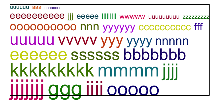

The word cloud is very basic. The words are ordered by the font sizes and are placed from the bottom to top. Words are assigned with random colors. There is a box that contains the word cloud. Here max_width argument controls the “maximal width” of the box. Note the final grob width returned by grobWidth(gb) might be a little bit smaller than the value specified with max_width because if the next word exceeds the box, it will be places into the next line in the box. I draw the border of the grob explicitly so that you can see the size of the grob.

If the width of the box changes, the height of the box changes accordingly. In the following example, the width is reduced to 60mm and you can see the box gets higher.

gb = word_cloud_grob(words, fontsize = fontsize, max_width = unit(60, "mm"))
grid.newpage()
grid.draw(gb)
grid.rect(width = grobWidth(gb), height = grobHeight(gb), gp = gpar(fill = NA))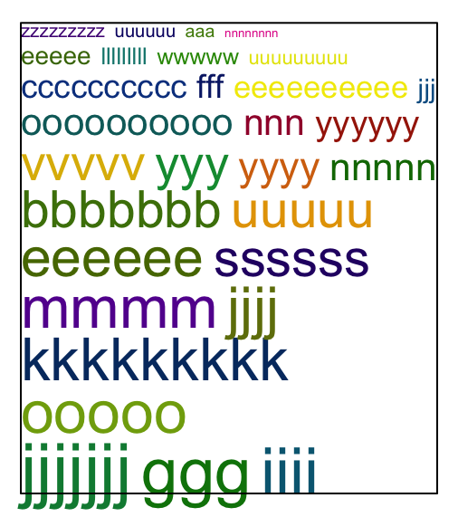

The colors of words help to distinguish between the words. The col argument can be set as a vector with the same length as the words.

# color as a vector
gb = word_cloud_grob(words, fontsize = fontsize, max_width = unit(100, "mm"), col = 1:30)
grid.newpage(); grid.draw(gb)
grid.rect(width = grobWidth(gb), height = grobHeight(gb), gp = gpar(fill = NA))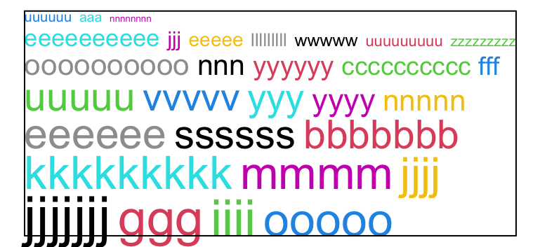

col can also be set as a color mapping function that maps from font sizes to colors. The color mapping function takes the fontsize vector as input and returns the corresponding colors.

# color as a function
library(circlize)
col_fun = colorRamp2(c(5, 17, 30), c("blue", "black", "red"))
gb = word_cloud_grob(words, fontsize = fontsize, max_width = unit(100, "mm"), 
    col = col_fun)
grid.newpage(); grid.draw(gb)
grid.rect(width = grobWidth(gb), height = grobHeight(gb), gp = gpar(fill = NA))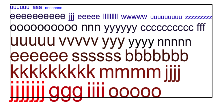

Other arguments in word_cloud_grob are line_space that controls the space between lines and word_space that controls the space between words.

As a heatmap annotation

anno_link() function links a subset of rows in the heatmap to an external viewport. The viewport that links to the heatmap should have fixed width and height. If the word cloud is taken as the annotation, the size of the viewport relates to the size of the word cloud grob. In the next code, I generated a word cloud grob and calcualte their height and width.

gb = word_cloud_grob(words, fontsize = fontsize, max_width = unit(100, "mm"))
gb_h = grobHeight(gb)
gb_w = grobWidth(gb)

I generate a random heatmap with 10 rows and 10 columns without row clustering, so that I can correspond the word cloud to the first three rows in the heatmap.

library(ComplexHeatmap)
m = matrix(rnorm(100), 10)
ht = Heatmap(m, cluster_rows = FALSE)

What to draw in the “linking viewport” should be manually defined. In the case here, I simply draw the word cloud by grid.draw(gb). I additionally draw the background of the word cloud in light grey.

panel_fun = function(index, nm) {
    grid.rect(gp = gpar(fill = "#EEEEEE", col = NA))
    grid.draw(gb)
}

anno_link() is set as follows. Note I also set the background color for the “linking line” same as the background of the word cloud.

ht + rowAnnotation(word_cloud = anno_link(align_to = 1:3, which = "row", 
        panel_fun = panel_fun, size = gb_h, 
        width = gb_w + unit(5, "mm"), # the link is 5mm
        link_gp = gpar(fill = "#EEEEEE", col = NA)
    ))

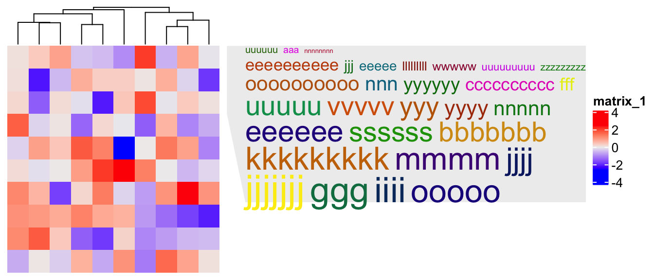
Ok, this is the simplest implementation of the word cloud annotation. To make it look nicer, you need to do a lot of manual adjustment. In the next section, I demonstrate how to make a nicer plot.

A real-world example

In this section, I reproduce the plot generated from simplifyEnrichment package. First I load some data objects:

tmp_file = tempfile()
download.file("https://jokergoo.github.io/word_cloud_annotation_example.RData", 
    destfile = tmp_file, quiet = TRUE)
load(tmp_file); file.remove(tmp_file)

There are following three objects:

mat A GO similarity matrix from 500 GO terms. Values are between 0 and 1 where 1 means exactly the same and 0 means completely different.
cl The clustering labels of the 500 GO terms.
keywords A list of keywords and their frequencies extracted from the GO names in the corresponding GO cluster.

The data structure or the values of the three objects are as follows:

mat[1:6, 1:6]

##            GO:0046654 GO:0060003 GO:0019918 GO:0006051 GO:0038016 GO:0045060
## GO:0046654 1.00000000  0.0000000 0.18082993 0.08979910 0.09389934 0.01450020
## GO:0060003 0.00000000  1.0000000 0.00000000 0.00000000 0.19300314 0.00000000
## GO:0019918 0.18082993  0.0000000 1.00000000 0.08408824 0.12754833 0.01349981
## GO:0006051 0.08979910  0.0000000 0.08408824 1.00000000 0.07906032 0.00000000
## GO:0038016 0.09389934  0.1930031 0.12754833 0.07906032 1.00000000 0.01262854
## GO:0045060 0.01450020  0.0000000 0.01349981 0.00000000 0.01262854 1.00000000

cl

##   [1] 1  2  1  1  2  3  4  5  1  5  1  1  5  4  5  6  6  3  3  5  3  3  3  1  3 
##  [26] 2  3  2  0  1  1  1  1  1  1  3  3  6  1  5  0  6  1  1  0  1  1  3  3  6 
##  [51] 1  5  3  6  3  2  2  1  3  3  0  2  3  3  2  6  11 5  2  3  0  4  5  1  13
##  [76] 3  2  1  5  3  1  6  6  3  1  3  1  6  1  3  1  1  11 2  3  0  1  1  1  1 
## [101] 3  2  1  1  2  15 1  16 2  5  1  0  13 5  1  6  5  5  5  0  3  1  3  1  3 
## [126] 6  2  6  1  3  3  3  3  2  6  1  1  1  3  11 5  5  3  1  5  1  1  3  3  3 
## [151] 1  1  3  2  3  3  0  2  1  1  2  5  0  2  6  1  5  1  1  6  5  2  0  3  15
## [176] 3  1  1  5  0  0  16 5  2  1  5  2  1  2  1  3  1  2  3  13 3  3  3  3  5 
## [201] 1  1  4  3  2  6  5  1  3  3  3  3  3  1  6  1  6  3  6  3  3  5  3  3  6 
## [226] 5  1  2  2  0  1  15 3  1  2  3  6  5  3  2  0  2  0  1  3  1  1  1  5  2 
## [251] 1  3  0  3  3  3  15 6  1  1  2  5  3  3  5  5  5  5  2  2  1  5  3  6  1 
## [276] 3  13 3  1  5  5  1  5  1  0  5  3  5  2  1  5  3  1  3  1  13 3  5  3  11
## [301] 3  1  2  1  2  15 6  15 2  3  6  4  3  5  1  1  13 3  1  1  3  0  5  1  5 
## [326] 2  5  3  3  2  2  1  0  3  5  3  5  0  6  5  0  2  5  2  5  2  1  1  16 6 
## [351] 1  1  11 5  1  1  2  5  5  2  2  6  1  3  0  13 2  3  6  1  1  1  2  6  1 
## [376] 5  2  5  0  5  3  1  0  3  5  3  5  5  3  6  5  5  3  0  16 3  3  2  1  1 
## [401] 2  3  4  0  3  1  1  1  16 0  1  3  3  3  5  0  2  0  6  3  1  2  1  1  5 
## [426] 3  2  16 2  2  6  5  3  0  3  5  0  2  5  6  3  5  1  3  3  5  3  5  1  5 
## [451] 3  2  15 2  2  5  5  5  3  1  3  4  3  3  0  1  5  1  0  3  3  1  5  3  2 
## [476] 1  3  1  3  1  2  3  1  4  1  0  2  3  16 2  1  3  1  5  3  2  1  6  2  1 
## Levels: 1 3 5 2 6 4 13 15 16 11 0

keywords

## $`1`
##                        word freq
## process             process   60
## regulation       regulation   47
## biosynthetic   biosynthetic   25
## metabolic         metabolic   20
## negative           negative   15
## positive           positive   13
## catabolic         catabolic   13
## activity           activity   11
## transcription transcription   10
## histone             histone    8
## 
## $`3`
##                            word freq
## regulation           regulation   40
## cell                       cell   38
## development         development   28
## differentiation differentiation   22
## positive               positive   20
## involved               involved   14
## morphogenesis     morphogenesis   11
## negative               negative   10
## formation             formation    7
## production           production    7
## 
## $`5`
##                  word freq
## response     response   39
## regulation regulation   25
## signaling   signaling   24
## pathway       pathway   21
## cellular     cellular   19
## receptor     receptor   11
## negative     negative    9
## cell             cell    7
## positive     positive    7
## stimulus     stimulus    6
## 
## $`2`
##                        word freq
## transport         transport   24
## regulation       regulation   23
## secretion         secretion   12
## ion                     ion    8
## localization   localization    7
## negative           negative    6
## transmembrane transmembrane    6
## vesicle             vesicle    6
## positive           positive    6
## cell                   cell    5
## 
## $`6`
##                      word freq
## regulation     regulation   17
## assembly         assembly   10
## organization organization    7
## cell                 cell    6
## mitotic           mitotic    6
## positive         positive    6
## cycle               cycle    5
## negative         negative    3
## complex           complex    3
## transition     transition    3
## 
## $`4`
##                  word freq
## apoptotic   apoptotic    6
## process       process    6
## regulation regulation    6
## cell             cell    3
## positive     positive    3
## negative     negative    2
## death           death    2
## 
## $`13`
##                        word freq
## proliferation proliferation    6
## regulation       regulation    6
## positive           positive    5
## cell                   cell    3
## muscle               muscle    2
## 
## $`15`
##                    word freq
## viral             viral    4
## regulation   regulation    3
## complex         complex    2
## host               host    2
## replication replication    2
## 
## $`16`
##                  word freq
## regulation regulation    5
## cell             cell    4
## adhesion     adhesion    4
## negative     negative    3
## positive     positive    2
## 
## $`11`
##                  word freq
## regulation regulation    5
## negative     negative    3
## binding       binding    3
## activity     activity    2
## positive     positive    2
## 
## $`0`
##                    word freq
## regulation   regulation   16
## positive       positive   11
## negative       negative    4
## antigen         antigen    4
## assembly       assembly    3
## homeostasis homeostasis    3
## calcium         calcium    3
## ion                 ion    3
## cell               cell    3
## presynapse   presynapse    2

I first define the similarity heatmap. The settings can be very straightforwardly understood from the argument names.

ht = Heatmap(mat, col = colorRamp2(c(0, 1), c("white", "red")),
    name = "Similarity",
    show_row_names = FALSE, show_column_names = FALSE,
    show_row_dend = FALSE, show_column_dend = FALSE,
    row_split = cl, column_split = cl, 
    border = "#404040", row_title = NULL, column_title = NULL,
    row_gap = unit(0, "mm"), column_gap = unit(0, "mm"))

There will be word clouds for every GO cluster, and since the GO terms are split by cl, the “alignment variable” is defined as follows. The GO cluster with label “0” is removed.

align_to = split(seq_len(nrow(mat)), cl)
align_to = align_to[names(align_to) != "0"]
align_to = align_to[names(align_to) %in% names(keywords)]
align_to

## $`1`
##   [1]   1   3   4   9  11  12  24  30  31  32  33  34  35  39  43  44  46  47
##  [19]  51  58  74  78  81  85  87  89  91  92  97  98  99 100 103 104 107 111
##  [37] 115 122 124 129 136 137 138 144 146 147 151 152 159 160 166 168 169 177
##  [55] 178 185 188 190 192 201 202 208 214 216 227 231 234 244 246 247 248 251
##  [73] 259 260 271 275 279 282 284 290 293 295 302 304 315 316 319 320 324 332
##  [91] 347 348 351 352 355 356 363 370 371 372 375 382 399 400 406 407 408 411
## [109] 421 423 424 443 449 460 466 468 472 476 478 480 483 485 491 493 497 500
## 
## $`3`
##   [1]   6  18  19  21  22  23  25  27  36  37  48  49  53  55  59  60  63  64
##  [19]  70  76  80  84  86  90  95 101 121 123 125 130 131 132 133 139 143 148
##  [37] 149 150 153 155 156 174 176 191 194 196 197 198 199 204 209 210 211 212
##  [55] 213 218 220 221 223 224 233 236 239 245 252 254 255 256 263 264 273 276
##  [73] 278 287 292 294 297 299 301 310 313 318 321 328 329 334 336 364 368 381
##  [91] 384 386 389 393 396 397 402 405 412 413 414 420 426 433 435 441 444 445
## [109] 447 451 459 461 463 464 470 471 474 477 479 482 488 492 495
## 
## $`5`
##  [1]   8  10  13  15  20  40  52  68  73  79 110 114 117 118 119 141 142 145 162
## [20] 167 171 179 183 186 200 207 222 226 238 249 262 265 266 267 268 272 280 281
## [39] 283 286 288 291 298 314 323 325 327 335 337 340 343 345 354 358 359 376 378
## [58] 380 385 387 388 391 392 415 425 432 436 439 442 446 448 450 456 457 458 467
## [77] 473 494
## 
## $`2`
##  [1]   2   5  26  28  56  57  62  65  69  77  94 102 105 109 127 134 154 158 161
## [20] 164 172 184 187 189 193 205 228 229 235 240 242 250 261 269 270 289 303 305
## [39] 309 326 330 331 342 344 346 357 360 361 367 373 377 398 401 417 422 427 429
## [58] 430 438 452 454 455 475 481 487 490 496 499
## 
## $`6`
##  [1]  16  17  38  42  50  54  66  82  83  88 116 126 128 135 165 170 206 215 217
## [20] 219 225 237 258 274 307 311 339 350 362 369 374 390 419 431 440 498
## 
## $`4`
## [1]   7  14  72 203 312 403 462 484
## 
## $`13`
## [1]  75 113 195 277 296 317 366
## 
## $`15`
## [1] 106 175 232 257 306 308 453
## 
## $`16`
## [1] 108 182 349 395 409 428 489
## 
## $`11`
## [1]  67  93 140 300 353

Next I construct a list of word cloud grob. Note I use scale_fontsize() to map word frequency to font size.

fontsize_range = c(4, 16)
gbl = lapply(names(align_to), function(nm) {
    kw = keywords[[nm]][, 1]
    freq = keywords[[nm]][, 2]
    fontsize = scale_fontsize(freq, rg = c(1, max(10, freq)), fs = fontsize_range)

    word_cloud_grob(text = kw, fontsize = fontsize)
})
names(gbl) = names(align_to)
gbl

## $`1`
## word_cloud[GRID.word_cloud.337] 
## 
## $`3`
## word_cloud[GRID.word_cloud.349] 
## 
## $`5`
## word_cloud[GRID.word_cloud.361] 
## 
## $`2`
## word_cloud[GRID.word_cloud.373] 
## 
## $`6`
## word_cloud[GRID.word_cloud.385] 
## 
## $`4`
## word_cloud[GRID.word_cloud.394] 
## 
## $`13`
## word_cloud[GRID.word_cloud.401] 
## 
## $`15`
## word_cloud[GRID.word_cloud.408] 
## 
## $`16`
## word_cloud[GRID.word_cloud.415] 
## 
## $`11`
## word_cloud[GRID.word_cloud.422]

I calculate the height of each word cloud and use the maximal width of all grob as the width of the “linking annotation”. The heights and widths are added with 8pt as margins.

margin = unit(8, "pt")
gbl_h = lapply(gbl, function(x) convertHeight(grobHeight(x), "cm") + margin)
gbl_h = do.call(unit.c, gbl_h)

gbl_w = lapply(gbl, function(x) convertWidth(grobWidth(x), "cm"))
gbl_w = do.call(unit.c, gbl_w)
gbl_w = max(gbl_w) + margin

The use of convertHeight() and convertWidth() is mainly for simplying the unit objects.

panel_fun is defined as follows. The use of grid.lines() only draws the bottom, right and top border of the viewport.

panel_fun = function(index, nm) {
    # background
    grid.rect(gp = gpar(fill = "#DDDDDD", col = NA))
    # border
    grid.lines(c(0, 1, 1, 0), c(0, 0, 1, 1), gp = gpar(col = "#AAAAAA"), 
        default.units = "npc")
    gb = gbl[[nm]]
    # a viewport within the margins
    pushViewport(viewport(x = margin/2, y = margin/2, 
        width = grobWidth(gb), height = grobHeight(gb),
        just = c("left", "bottom")))
    grid.draw(gb)
    popViewport()
}

And the final heatmap with the word cloud annotations are as follows.

ht = ht + rowAnnotation(keywords = anno_link(align_to = align_to, 
    which = "row", panel_fun = panel_fun, 
    size = gbl_h, gap = unit(2, "mm"), 
    width = gbl_w + unit(5, "mm"), # 5mm for the link
    link_gp = gpar(fill = "#DDDDDD", col = "#AAAAAA"), 
    internal_line = FALSE)) # you can set it to TRUE to see what happens
draw(ht, ht_gap = unit(2, "pt"))