Guillaume Devailly recently wrote an article on image rasterization to efficiently visualize huge matrices in R, as well as comparing several R functions that support image rasterization. In this post, I discusse the support for raster image in ComplexHeatmap in more details.
When we produce so-called “high quality figures”, normally we save the figures as vector graphics in the format of e.g. pdf or svg. The vector graphics basically store details of every single graphic elements, thus, if a heatmap made from a very huge matrix is saved as vector graphics, the final file size would be very big. On the other hand, when visualizing e.g. the pdf file on the screen, multiple grids from the heatmap actually only map to single pixels, due to the limited size of the screen. Thus, there need some ways to effectively reduce the original image and it is not necessary to store the complete matrix for the heatmap.
Rasterization is a way to covnert the vector graphics into a matrix of colors. In this case, an image is represented as a matrix of RGB values, which is called a raster image. If the heatmap is larger than the size of the screen or the pixels that current graphics devices can support, we can convert the heatmap and reduce it, by saving it in a form of a color matrix with the same dimension as the device.
Let’s assume a matrix has \(n_r\) rows and \(n_c\) columns. When it is drawn on a certain graphics device, e.g. an on-screen device, the corresponding heatmap body has \(p_r\) and \(p_c\) pixels (or points) for the rows and columns, respectively. When \(n_r > p_r\) and/or \(n_c > p_c\), multiple values in the matrix are mapped to single pixels. Here we need to reduce \(n_r\) and/or \(n_c\) if they are larger than \(p_r\) and/or \(p_c\).
To make it simple, I assume both \(n_r > p_r\) and \(n_c > p_c\). The principle is basically the same for the scenarios where only one dimension of the matrix is larger than the device.
In ComplexHeatmap version 2.5.4, there are following implementations for image rasterization. Note the implementation is a little bit different from the earlier versions (of course, better than the earlier versions).
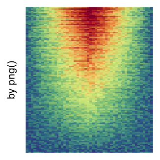
First an image (in a specific format, e.g. png or jpeg) with \((p_r \cdot a) \times (p_c \cdot a)\) resolution is saved into a temporary file where \(a\) is a zooming factor, next it is read back as a
rasterobject by e.g.png::readPNG()orjpeg::readJPEG(), and later the raster object is filled into the heatmap body bygrid::grid.raster(). So we can say, the rasterization is done by the raster image devices (png()orjpeg()).This type of rasterization is automatically turned on (if magick package is not installed) when the number of rows or columns exceeds 2000 (You will see a message. It won’t happen silently). It can also be manually controlled by setting the
use_rasterargument:
Heatmap(..., use_raster = TRUE)The zooming factor is controlled by raster_quality argument. A value larger
than 1 generates files with larger size.
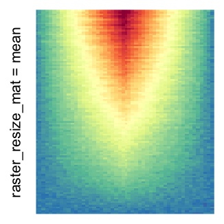
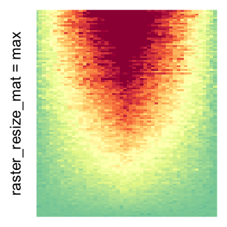
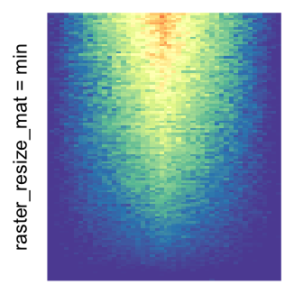
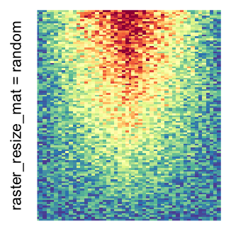
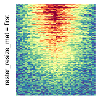
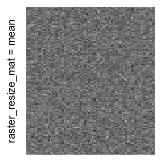
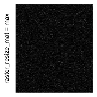
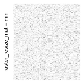
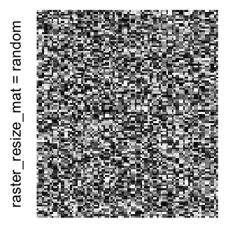
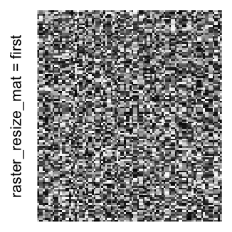
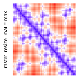
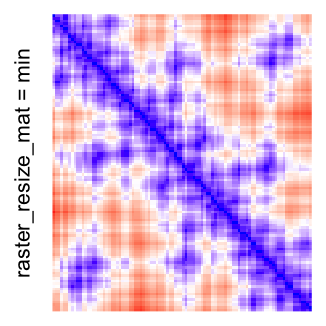
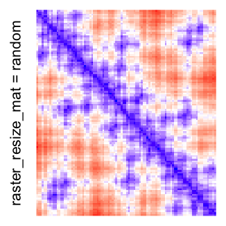
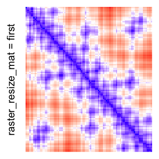
Heatmap(..., use_raster = TRUE, raster_quality = 5)Simply reduce the original matrix to \(p_r \times p_c\) where now each single values can correspond to single pixels. In the reduction, a user-defined function is applied to summarize the sub-matrices.
This can be set by
raster_resize_matargument:
# the default summary function is mean()
Heatmap(..., use_raster = TRUE, raster_resize_mat = TRUE)
# use max() as the summary function
Heatmap(..., use_raster = TRUE, raster_resize_mat = max)
# randomly pick one
Heatmap(..., use_raster = TRUE, raster_resize_mat = function(x) sample(x, 1))
A temporary image with resolution \(n_r \times n_c\) is first generated, here
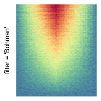
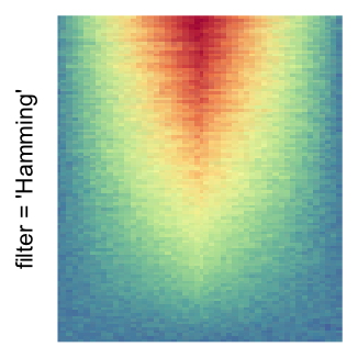
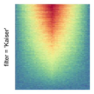
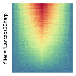
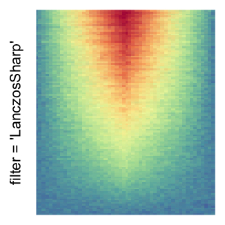
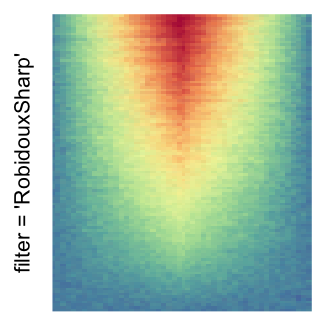
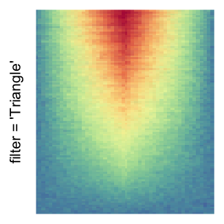
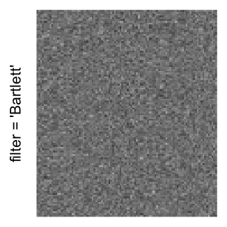
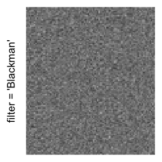
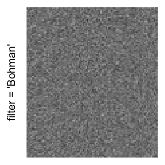
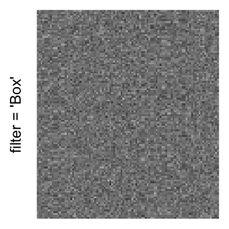
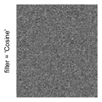
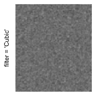
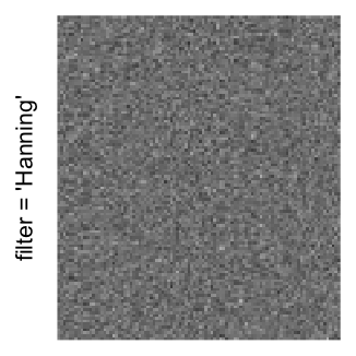
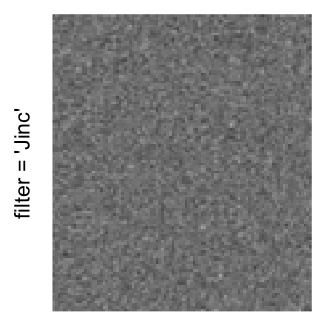
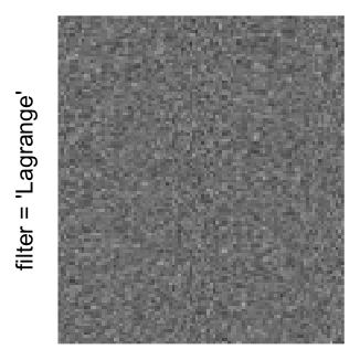
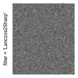
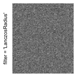
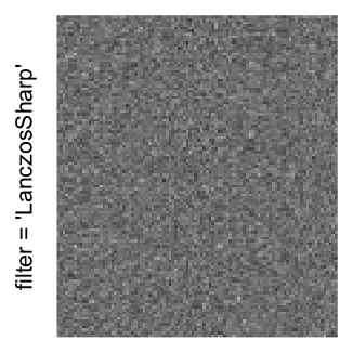
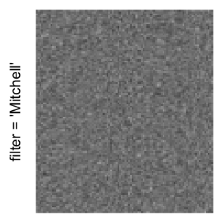
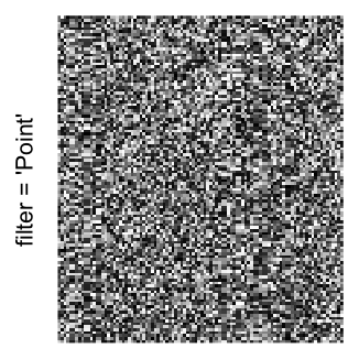
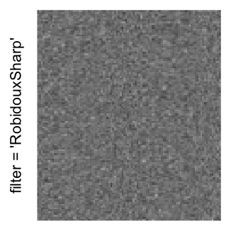
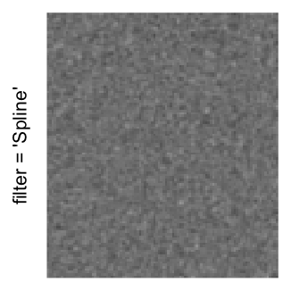
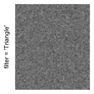
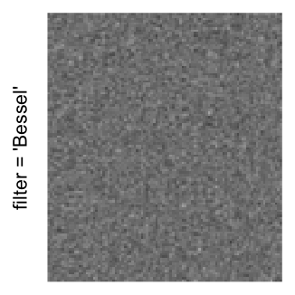
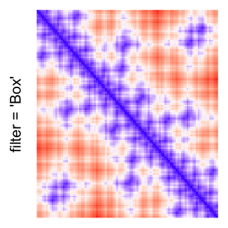
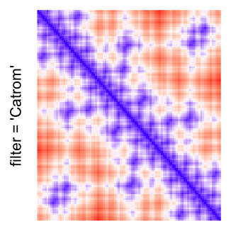
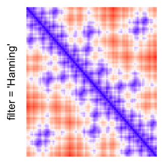
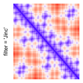
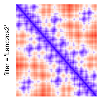
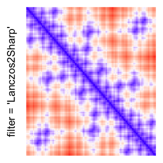
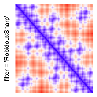
magick::image_resize()is used to reduce the image to size \(p_r \times p_c\). Finally the reduced image is read as arasterobject and filled into the heatmap body. magick provides a lot of methods for “resizing”/“scaling” the image, which is called the “filtering methods” under the term of magick. All filtering methods can be obtained bymagick::filter_types().This type of rasterization can be truned on by setting
raster_by_magick = TRUEand choosing a properraster_magick_filter.
Heatmap(..., use_raster = TRUE, raster_by_magick = TRUE)
Heatmap(..., use_raster = TRUE, raster_by_magick = TRUE, raster_magick_filter = ...)
In the following parts of this post, I will compare the visual difference between different image rasterization methods.
Example 1
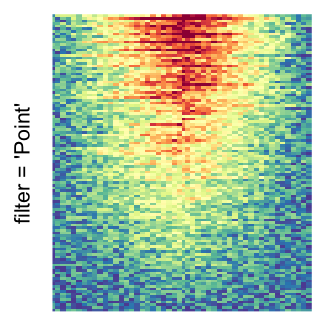
The first example is from Guillaume Devailly’s simulated data but with small adaptation. This example shows an enrichment pattern to the top center of the plot.
mat = matrix(nrow = 5000, ncol = 50)
for(i in 1:5000) {
    mat[i, ] = runif(50) + c(sort(abs(rnorm(50)))[1:25], rev(sort(abs(rnorm(50)))[1:25]))  * i/1000
}
mat = mat[nrow(mat):1, ]
col_fun = colorRamp2(seq(quantile(mat, 0.01), quantile(mat, 0.99), len = 11), rev(brewer.pal(11, "Spectral")))
In the folowing examples, I won’t show the code for making heatmaps because there are too many heatmaps and the specific settings is already written as the row title of each heatmap.
I set the same color mapping for all heatmaps, so that you can see how different rasterizations change the original patterns.
For the comparison, I generated many heatmaps. They can be categoried into three groups, as corresponded to the three rasterization methods I mentioned previously.
by png(): Rasterization method 1.raster_resize_mat = *: Rasterization method 2, with different summary methods.filter = *: Rasterization method 3, with different filterring method. The stringfiltershould beraster_magick_filter. It is truncated so that the row title won’t be cut by the plot regions.


Example 2
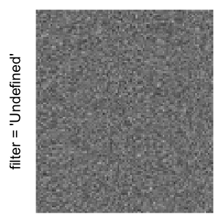
Here we generate a random matrix from uniform distribution. The color mapping function linearly intepolation colors between 0 and 1 in the sRGB color space.
set.seed(123)
mat = matrix(runif(2000*100), nrow = 2000)
col_fun = colorRamp2(c(0, 1), c("white", "black"), space = "sRGB")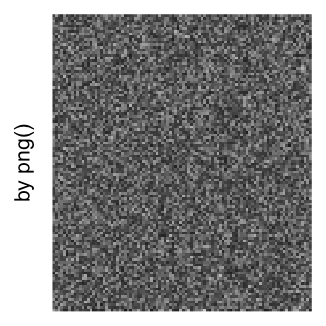


Example 3
This example shows heatmaps with more local patterns. These heatmaps visualize the distance of points in a 2D Hilbert curve.
pos = HilbertVis::hilbertCurve(5)
mat = as.matrix(dist(pos))
dimnames(mat) = NULL
col_fun = colorRamp2(c(min(mat), median(mat), max(mat)), c("blue", "white", "red"))


Example 4
This example shows a pattern only on the diagonal of the matrix. The matrix is also from Guillaume Devailly’s eQTL data, but only a small subset of 2000 rows and columns are used.
mat = readRDS("~/eqtl_small_matrix.rds")
dimnames(mat) = NULL
col_fun = colorRamp2(c(0, quantile(mat, 0.95)*0.5, quantile(mat, 0.95)), c("white", "darkorange", "black"))
Conclusion
According to all these examples that have been shown, I would say
rasterization by magick package performs better, thus, by default, in
ComplexHeatmap, the rasterization is done by magick (with "Lanczos"
as the default filter method) and if magick is not installed, it uses
png() and a friendly message is printed to suggest users to install
magick.