There are some scenarios where users want to visualize more than one genomes in the circular plots. This can be done by making “a combined genome”. In the following example, I combine both human and mouse genomes.
library(circlize)
human_cytoband = read.cytoband(species = "hg19")$df
mouse_cytoband = read.cytoband(species = "mm10")$df
One thing important is since the two genome will be combined, the chromosome
names for each genome need to be adjusted. Here I simply add human_/mouse_
prefix.
human_cytoband[ ,1] = paste0("human_", human_cytoband[, 1])
mouse_cytoband[ ,1] = paste0("mouse_", mouse_cytoband[, 1])
Now I can combine the two cytoband data frames into one.
cytoband = rbind(human_cytoband, mouse_cytoband)
head(cytoband)
## V1 V2 V3 V4 V5
## 1 human_chr1 0 2300000 p36.33 gneg
## 2 human_chr1 2300000 5400000 p36.32 gpos25
## 3 human_chr1 5400000 7200000 p36.31 gneg
## 4 human_chr1 7200000 9200000 p36.23 gpos25
## 5 human_chr1 9200000 12700000 p36.22 gneg
## 6 human_chr1 12700000 16200000 p36.21 gpos50The combined cytoband is still a valid cytoband data frame, thus, the ideograms
can be drawn for the combined genome. Also when I construct the variable chromosome.index,
I let human chromosome 1 to be close to mouse chromosome 1.
chromosome.index = c(paste0("human_chr", c(1:22, "X", "Y")),
                     rev(paste0("mouse_chr", c(1:19, "X", "Y"))))
circos.initializeWithIdeogram(cytoband, chromosome.index = chromosome.index)
circos.clear()By default, in the plot there are chromosome names, axes and ideograms. Now
for the combined genome, since there are quite a lot of chromosomes, each
chromosome will be very short in the plot, which makes it not easy to read the
axes and the long chromosome names. In the following improved code, I turn off
the chromosome name and the axes. We create a small track to discriminate
human chromosomes and mouse chromosomes (by highlight.chromosome()) and I
only write the numeric indices (also X and Y) for chromosomes. A gap of 5
degrees is set between human and mouse chromosomes (by
circos.par("gap.after")).
circos.par(gap.after = c(rep(1, 23), 5, rep(1, 20), 5))
circos.initializeWithIdeogram(cytoband, plotType = NULL,
    chromosome.index = chromosome.index)
circos.track(ylim = c(0, 1), panel.fun = function(x, y) {
    circos.text(CELL_META$xcenter, CELL_META$ylim[2] + mm_y(2),
        gsub(".*chr", "", CELL_META$sector.index), cex = 0.6, niceFacing = TRUE)
}, track.height = mm_h(1), cell.padding = c(0, 0, 0, 0), bg.border = NA)
highlight.chromosome(paste0("human_chr", c(1:22, "X", "Y")),
    col = "red", track.index = 1)
highlight.chromosome(paste0("mouse_chr", c(1:19, "X", "Y")),
    col = "blue", track.index = 1)

circos.genomicIdeogram(cytoband)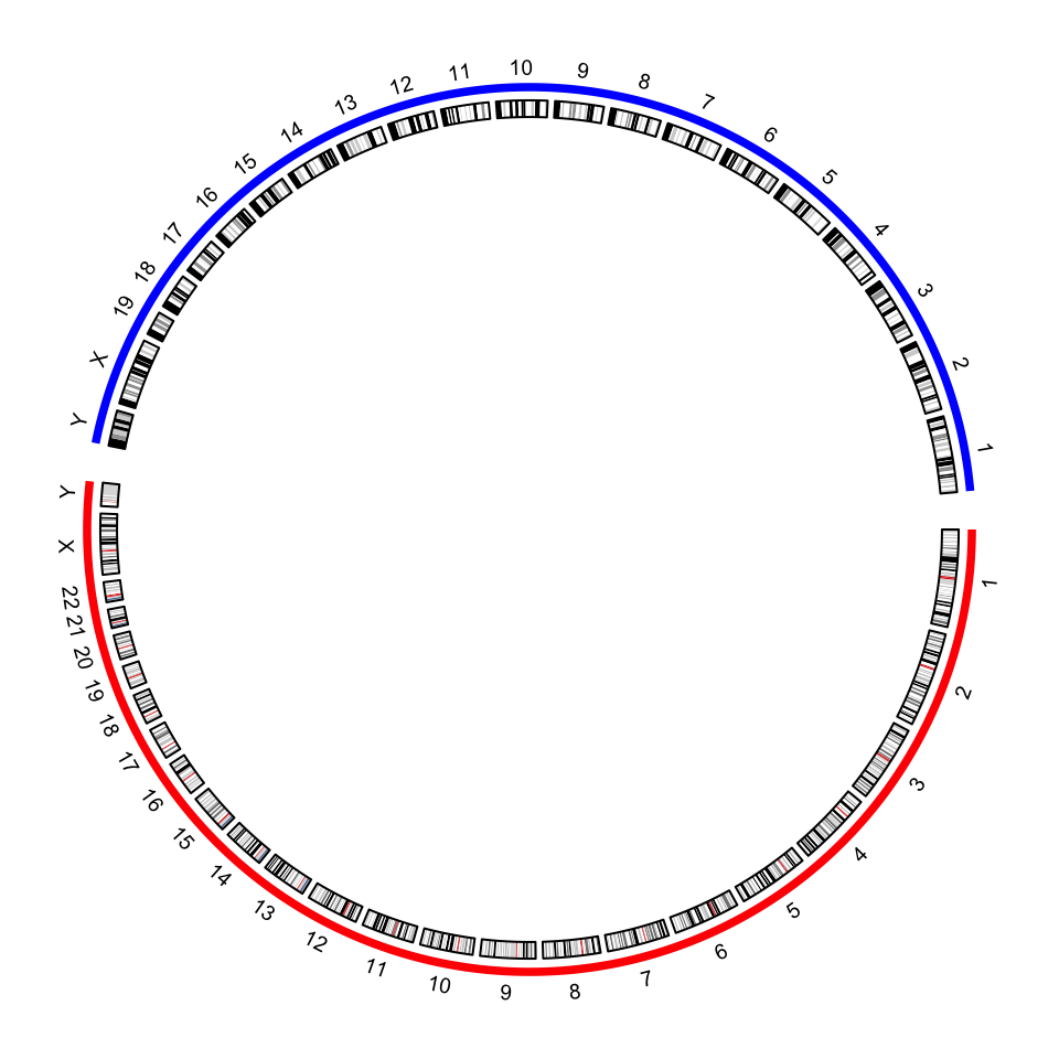
circos.clear()In previous example, I demonstrate to create the circular layout for the
combined genome with the cytoband data frames. The layout can also be created
only by the chromosome ranges, i.e., the length of each chromosome. In the
following code, read.chromInfo() can fetch the chromosome range for a
specific genome.
human_chromInfo = read.chromInfo(species = "hg19")$df
mouse_chromInfo = read.chromInfo(species = "mm10")$df
human_chromInfo[ ,1] = paste0("human_", human_chromInfo[, 1])
mouse_chromInfo[ ,1] = paste0("mouse_", mouse_chromInfo[, 1])
chromInfo = rbind(human_chromInfo, mouse_chromInfo)
# note the levels of the factor controls the chromosome orders in the plot
chromInfo[, 1] = factor(chromInfo[ ,1], levels = chromosome.index)
head(chromInfo)
## chr start end
## 1 human_chr1 0 249250621
## 2 human_chr2 0 243199373
## 3 human_chr3 0 198022430
## 4 human_chr4 0 191154276
## 5 human_chr5 0 180915260
## 6 human_chr6 0 171115067With the specified chromosome ranges, circos.genomicInitialize() is used to initialize the
layout.
circos.par(gap.after = c(rep(1, 23), 5, rep(1, 20), 5))
circos.genomicInitialize(chromInfo, plotType = NULL)
circos.track(ylim = c(0, 1), panel.fun = function(x, y) {
    circos.text(CELL_META$xcenter, CELL_META$ylim[2] + mm_y(2),
        gsub(".*chr", "", CELL_META$sector.index), cex = 0.6, niceFacing = TRUE)
}, track.height = mm_h(1), cell.padding = c(0, 0, 0, 0), bg.border = NA)
highlight.chromosome(paste0("human_chr", c(1:22, "X", "Y")),
    col = "red", track.index = 1)
highlight.chromosome(paste0("mouse_chr", c(1:19, "X", "Y")),
    col = "blue", track.index = 1)

circos.track(ylim = c(0, 1))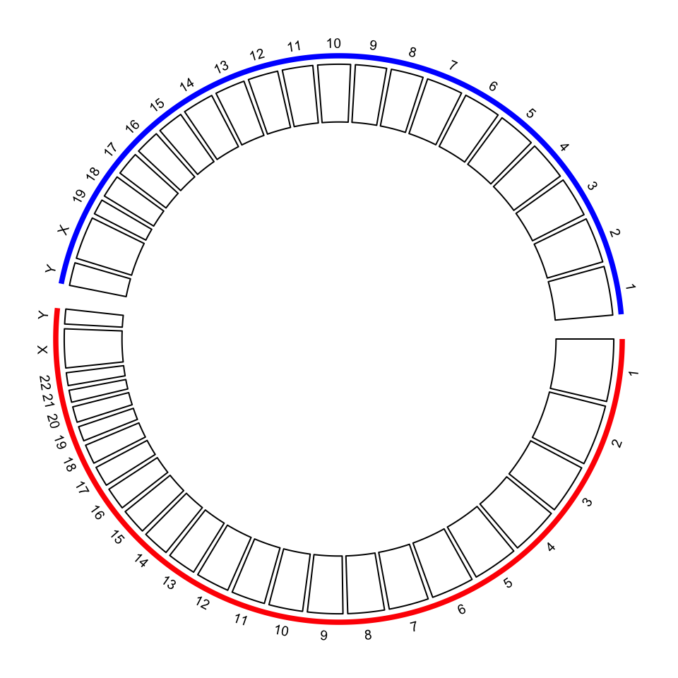
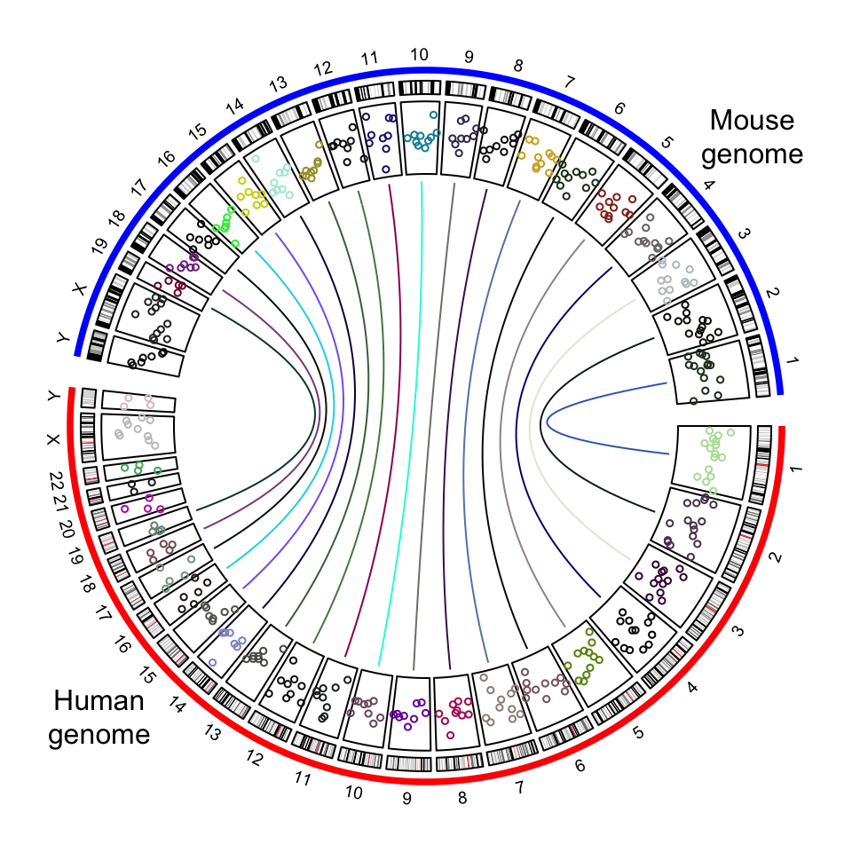
circos.clear()Adding more tracks has no difference to the single-genome plots. The only thing to note is the chromosome names should be properly formatted. In the following code, I create a track of points and add links between human and mouse genomes.
circos.par(gap.after = c(rep(1, 23), 5, rep(1, 20), 5))
circos.genomicInitialize(chromInfo, plotType = NULL)
circos.track(ylim = c(0, 1), panel.fun = function(x, y) {
    circos.text(CELL_META$xcenter, CELL_META$ylim[2] + mm_y(2),
        gsub(".*chr", "", CELL_META$sector.index), cex = 0.6, niceFacing = TRUE)
}, track.height = mm_h(1), cell.padding = c(0, 0, 0, 0), bg.border = NA)
highlight.chromosome(paste0("human_chr", c(1:22, "X", "Y")),
    col = "red", track.index = 1)
highlight.chromosome(paste0("mouse_chr", c(1:19, "X", "Y")),
    col = "blue", track.index = 1)

circos.genomicIdeogram(cytoband)

# a track of points
human_df = generateRandomBed(200, species = "hg19")
mouse_df = generateRandomBed(200, species = "mm10")
human_df[ ,1] = paste0("human_", human_df[, 1])
mouse_df[ ,1] = paste0("mouse_", mouse_df[, 1])
df = rbind(human_df, mouse_df)
circos.genomicTrack(df, panel.fun = function(region, value, ...) {
    circos.genomicPoints(region, value, col = rand_color(1), cex = 0.5, ...)
})

# links between human and mouse genomes
human_mid = data.frame(
    chr = paste0("human_chr", 1:19),
    mid = round((human_chromInfo[1:19, 2] + human_chromInfo[1:19, 3])/2)
)
mouse_mid = data.frame(
    chr = paste0("mouse_chr", 1:19),
    mid = round((mouse_chromInfo[1:19, 2] + mouse_chromInfo[1:19, 3])/2)
)
circos.genomicLink(human_mid, mouse_mid, col = rand_color(19))
circos.clear()
text(-0.9, -0.8, "Human\ngenome")
text(0.9, 0.8, "Mouse\ngenome")