In this post, I will simply demonstrate how to visualize lift overs between two assemblies.
In the package rtracklayer, there is a function liftOver() that can convert genomic regions
according to the mapping encoded in a “chain” file.
In the following code, I will demonstrate the lift overs from hg19 to hg38. I first download
the chain file from UCSC database. Note the .gz file needs to be uncompressed.
library(glue)
chain_file = "https://hgdownload.soe.ucsc.edu/gbdb/hg19/liftOver/hg19ToHg38.over.chain.gz"
chain_file_basename = basename(chain_file)
tmp_dir = tempdir()
local_file = glue("{tmp_dir}/{chain_file_basename}")
download.file(chain_file, destfile = local_file)
system(glue("gzip -d -f '{local_file}'"))
Simply use import.chain() to create a Chain object.
library(rtracklayer)
chain = import.chain(gsub("\\.gz$", "", local_file))
To establish the correspondance between hg19 and hg38, I split hg19 assembly by 5kb windows
and I look for their corresponding regions in hg38.
Here read.chromInfo() returns the chromosome lengths of a genome. Of course you can use other ways
to obtain such information, such as GenomicFeatures::getChromInfoFromUCSC("hg19").
library(circlize)
genome_df = read.chromInfo(species = "hg19")$df
genome_gr = GRanges(seqnames = genome_df[, 1], ranges = IRanges(genome_df[, 2]+1, genome_df[, 3]))
And I split the genome by 5kb window.
library(EnrichedHeatmap)
genome_bins = makeWindows(genome_gr, w = 5000)
Now I do the lift over. In liftOver(), I simply provide the regions in hg19 and the Chain object.
to_bins = liftOver(genome_bins, chain)
to_bins
## GRangesList object of length 619122:
## [[1]]
## GRanges object with 0 ranges and 2 metadata columns:
## seqnames ranges strand | .i_query .i_window
## <Rle> <IRanges> <Rle> | <integer> <integer>
## -------
## seqinfo: 24 sequences from an unspecified genome; no seqlengths
##
## [[2]]
## GRanges object with 0 ranges and 2 metadata columns:
## seqnames ranges strand | .i_query .i_window
## <Rle> <IRanges> <Rle> | <integer> <integer>
## -------
## seqinfo: 24 sequences from an unspecified genome; no seqlengths
##
## [[3]]
## GRanges object with 1 range and 2 metadata columns:
## seqnames ranges strand | .i_query .i_window
## <Rle> <IRanges> <Rle> | <integer> <integer>
## [1] chr1 10001-15000 * | 1 3
## -------
## seqinfo: 24 sequences from an unspecified genome; no seqlengths
##
## ...
## <619119 more elements>To reduce the numbers of mapped regions, if there are multiple regions in hg38 are mapped to the same 5kb window in hg19, if the gap between then is less than 500bp, I just merge them. Also there might be some 5kb windows in hg19 have no mapping in hg38. In the following code, I just remove these 5kb windows in hg19 having no mapping in hg38.
to_bins = reduce(to_bins, min = 500)
n = sapply(start(to_bins), length)
l = n > 0
to_bins = to_bins[l]
genome_bins = genome_bins[l]
Now genome_bin contains a list of 5kb windows in hg19 and to_bins contains the mappings in hg38.
To visualize the relationships, I convert both objects to data frames. It is very easy to convert genome_bin to a data frame.
df_from = as.data.frame(genome_bins)[, 1:3]to_bins is a GRanegsList object because a 5kb window in hg19 may map to multiple regions in hg38. To simplify
the task, if a 5kb window in hg19 maps to multiple regions in hg38, I only use the first one.
It is not easy to get the chromosome name of the first region in every mapping. You can do
sapply(sq, function(x) as.vector(x)[1]), but it is actually very slow. In the
following code, I use the internal function PartitioningByEnd() to get the the index
of every first chromosome.
sq = seqnames(to_bins)
pa = PartitioningByEnd(sq)
df_to = data.frame(
    chr = as.vector(unlist(sq))[start(pa)],
    start = sapply(start(to_bins), function(x) x[1]),
    end = sapply(end(to_bins), function(x) x[1])
)
I restrict the chromosomes to “normal chromosomes”:
from_chromosomes = paste0("chr", c(1:22, "X", "Y"))
to_chromosomes = paste0("chr", c(1:22, "X", "Y"))

l = df_from[, 1] %in% from_chromosomes & df_to[, 1] %in% to_chromosomes
df_from = df_from[l, ]
df_to = df_to[l, ]
Now let’s check the value of df_from (hg19) and df_to (hg38):
head(df_from)## seqnames start end
## 1 chr1 10001 15000
## 2 chr1 15001 20000
## 3 chr1 20001 25000
## 4 chr1 25001 30000
## 5 chr1 30001 35000
## 6 chr1 35001 40000head(df_to)## chr start end
## 1 chr1 10001 15000
## 2 chr1 15001 20000
## 3 chr1 20001 25000
## 4 chr1 25001 30000
## 5 chr1 30001 35000
## 6 chr1 35001 40000And the number of regions remains:
nrow(df_from)## [1] 572281nrow(df_to)## [1] 572281The data is ready, next I can make the circular plot. I first extract the chromosome lengths for both assemblies.
from_chromInfo = read.chromInfo(species = "hg19")$df
from_chromInfo = from_chromInfo[from_chromInfo[, 1] %in% from_chromosomes, ]

to_chromInfo = read.chromInfo(species = "hg38")$df
to_chromInfo = to_chromInfo[to_chromInfo[, 1] %in% to_chromosomes, ]
Since I will put two assemblies in one plot, and the two assemblies are all for human,
I add prefix "from_" and "to_" to distinguish them.
from_chromInfo[ ,1] = paste0("from_", from_chromInfo[, 1])
to_chromInfo[ ,1] = paste0("to_", to_chromInfo[, 1])
chromInfo = rbind(from_chromInfo, to_chromInfo)
Similiarly, I add the prefix to df_from and df_to.
df_from[, 1] = paste0("from_", df_from[, 1])
df_to[, 1] = paste0("to_", df_to[, 1])
chromInfo contains chromosome lengths for both hg19 and hg38 and it can be thought as a “combined” genome,
where e.g. "from_chr1" and "to_chr1" are two different chromosomes. In the final circular plot, for easy correspondance
between two assemblies, I will let chr1 for both assemblies close in the plot and chrX/chrY also close in the plot.
In this case, I need to manually control the chromosome orders.
I just need to reverse the order of to_chromosomes. The chromosome orders are encoded as “levels” of the first column
in chromInfo.
chromosome.index = c(paste0("from_", from_chromosomes), paste0("to_", rev(to_chromosomes)))
chromInfo[, 1] = factor(chromInfo[ ,1], levels = chromosome.index)
Next I use circlize package to visualize the lift overs. If you know circlize, the following code is very straightforward to understand. Note here I randomly sampled 10000 regions for visualization.
library(circlize)
circos.par(gap.after = c(rep(1, length(from_chromosomes) - 1), 5, rep(1, length(to_chromosomes) - 1), 5))
circos.genomicInitialize(chromInfo, plotType = NULL)

circos.track(ylim = c(0, 1), panel.fun = function(x, y) {
    circos.text(CELL_META$xcenter, CELL_META$ylim[2] + mm_y(2),
        gsub(".*chr", "", CELL_META$sector.index), cex = 0.6, niceFacing = TRUE)
}, track.height = mm_h(1), cell.padding = c(0, 0, 0, 0), bg.border = NA)

circos.track(ylim = c(0, 1), cell.padding = c(0, 0, 0, 0), bg.border = NA, bg.col = "grey", track.height = mm_h(1))

highlight.chromosome(paste0("from_", from_chromosomes), col = "red", track.index = 1)
highlight.chromosome(paste0("to_", to_chromosomes), col = "blue", track.index = 1)

ind = sample(nrow(df_from), 10000)
col = rand_color(length(to_chromosomes))
names(col) = paste0("to_", to_chromosomes)
circos.genomicLink(df_from[ind, ], df_to[ind, ], col = add_transparency(col[df_to[ind, 1]], 0.9))

circos.clear()

text(0.9, -0.9, "hg19")
text(0.9, 0.9, "hg38")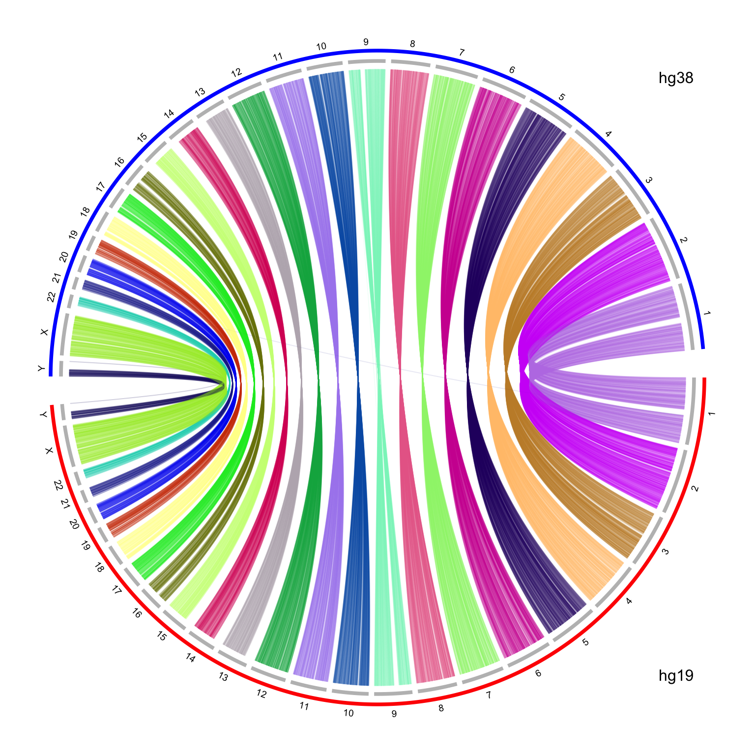
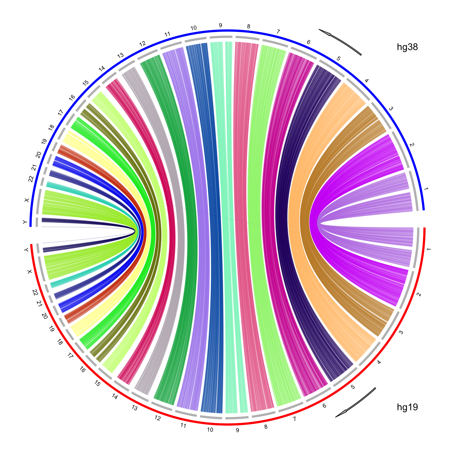
It looks nice, but there is one limit in the plot. I reversed the chromosome order for hg38 which are on the top half of the circle. The chromosomes for hg38 are reverse clockwise, but the x-axes on the hg38 chromosomes are still clockwise, which makes the links twisted. To improve the visualization, I manually reverse the x-axes of hg38 chromosomes with a simple transformation by the following code:
# `to` genome is put on the top of the circle, where the x-axis is reversed
gsize = structure(chromInfo[, 3], names = as.vector(chromInfo[, 1]))
df_to[, 2] = gsize[df_to[, 1]] - df_to[, 2]
df_to[, 3] = gsize[df_to[, 1]] - df_to[, 3]
df_to[, 2:3] = df_to[, 3:2]
I make the plot with the same code, and I explicitely add two arrows to represent the directions of x-axes. Now it looks better!
Finally I have wrapped the code into a function which can be found at https://gist.github.com/jokergoo/4161997c2a60ac90ae57017b19aea81e.
In the function viz_lift_over() you just specifiy two genome IDs, e.g.,
viz_lift_over("mm9", "mm10")Session info
sessionInfo()## R version 4.2.0 (2022-04-22)
## Platform: x86_64-apple-darwin17.0 (64-bit)
## Running under: macOS Big Sur/Monterey 10.16
##
## Matrix products: default
## BLAS: /Library/Frameworks/R.framework/Versions/4.2/Resources/lib/libRblas.0.dylib
## LAPACK: /Library/Frameworks/R.framework/Versions/4.2/Resources/lib/libRlapack.dylib
##
## locale:
## [1] C/UTF-8/C/C/C/C
##
## attached base packages:
## [1] grid stats4 stats graphics grDevices utils datasets
## [8] methods base
##
## other attached packages:
## [1] EnrichedHeatmap_1.26.0 ComplexHeatmap_2.13.2 circlize_0.4.16
## [4] rtracklayer_1.56.1 GenomicRanges_1.48.0 GenomeInfoDb_1.32.2
## [7] IRanges_2.30.0 S4Vectors_0.34.0 BiocGenerics_0.42.0
## [10] glue_1.6.2 knitr_1.39 colorout_1.2-2
##
## loaded via a namespace (and not attached):
## [1] locfit_1.5-9.6 Rcpp_1.0.9
## [3] lattice_0.20-45 png_0.1-7
## [5] Rsamtools_2.12.0 Biostrings_2.64.0
## [7] digest_0.6.29 foreach_1.5.2
## [9] R6_2.5.1 evaluate_0.15
## [11] highr_0.9 blogdown_1.10
## [13] GlobalOptions_0.1.2 zlibbioc_1.42.0
## [15] rlang_1.0.4 jquerylib_0.1.4
## [17] GetoptLong_1.1.0 Matrix_1.4-1
## [19] rmarkdown_2.14 BiocParallel_1.30.3
## [21] stringr_1.4.0 RCurl_1.98-1.8
## [23] DelayedArray_0.22.0 compiler_4.2.0
## [25] xfun_0.31 shape_1.4.6
## [27] htmltools_0.5.3 SummarizedExperiment_1.26.1
## [29] GenomeInfoDbData_1.2.8 bookdown_0.27
## [31] codetools_0.2-18 matrixStats_0.62.0
## [33] XML_3.99-0.10 crayon_1.5.1
## [35] GenomicAlignments_1.32.1 bitops_1.0-7
## [37] jsonlite_1.8.0 magrittr_2.0.3
## [39] cli_3.3.0 stringi_1.7.8
## [41] cachem_1.0.6 XVector_0.36.0
## [43] doParallel_1.0.17 bslib_0.4.0
## [45] rjson_0.2.21 restfulr_0.0.15
## [47] RColorBrewer_1.1-3 iterators_1.0.14
## [49] tools_4.2.0 Biobase_2.56.0
## [51] MatrixGenerics_1.8.1 parallel_4.2.0
## [53] fastmap_1.1.0 yaml_2.3.5
## [55] clue_0.3-61 colorspace_2.0-3
## [57] cluster_2.1.3 sass_0.4.2
## [59] BiocIO_1.6.0