Links in circos plot can show relations between elements. In most cases, links are drawn in the most inside of the circle. However, separating links into two categories of those having short distances and those having large distances, and distinguishing them by putting them onto different sides of a track can sometimes improve the visualization. One typical example is to separate intergenic translocations and intragenic translocations of genes.
In the next example, I first generate positions for three genes (A, B, and C).
Note for simplicity, the positions are not really bases.
set.seed(123)
x = sort(runif(20))
df1 = data.frame(x1 = x[1:20 %% 2 == 0], x2 = x[1:20 %% 2 == 1])
df1 = cbind(gene = "A", df1)

x = sort(runif(10, max = 0.5))
df2 = data.frame(x1 = x[1:10 %% 2 == 0], x2 = x[1:10 %% 2 == 1])
df2 = cbind(gene = "B", df2)

x = sort(runif(30, max = 2))
df3 = data.frame(x1 = x[1:30 %% 2 == 0], x2 = x[1:30 %% 2 == 1])
df3 = cbind(gene = "C", df3)

df = rbind(df1, df2, df3)
df
## gene x1 x2
## 1 A 0.04555650 0.04205953
## 2 A 0.24608773 0.10292468
## 3 A 0.32792072 0.28757752
## 4 A 0.45333416 0.40897692
## 5 A 0.52810549 0.45661474
## 6 A 0.57263340 0.55143501
## 7 A 0.78830514 0.67757064
## 8 A 0.89241904 0.88301740
## 9 A 0.94046728 0.89982497
## 10 A 0.95683335 0.95450365
## 11 B 0.14457987 0.07355682
## 12 B 0.29707101 0.27203301
## 13 B 0.32785290 0.32025341
## 14 B 0.35426523 0.34640170
## 15 B 0.49713489 0.44476966
## 16 C 0.09166233 0.04922737
## 17 C 0.25506330 0.24379852
## 18 C 0.28560004 0.27761213
## 19 C 0.41306278 0.30488950
## 20 C 0.46325157 0.43281587
## 21 C 0.53194528 0.46606820
## 22 C 0.73769090 0.63636202
## 23 C 0.82744865 0.74892555
## 24 C 0.88440015 0.82909267
## 25 C 0.95559194 0.93192490
## 26 C 1.38141056 1.12189597
## 27 C 1.51691908 1.50661573
## 28 C 1.59784969 1.59093484
## 29 C 1.79009072 1.71565543
## 30 C 1.92604847 1.80459809I also generate the relations of translocation positions on the three genes. There are intragenic translocations where the translocation happens in the same gene, and intergenic translocations where the translocation happens in different genes.
link = data.frame(
    gene1 = sample(c("A", "B", "C"), nrow(df), replace = TRUE),
    x1 = 0,
    gene2 = sample(c("A", "B", "C"), nrow(df), replace = TRUE),
    x2 = 0
)
for(i in seq_len(nrow(link))) {
    if(link$gene1[i] == "A") {
        link$x1[i] = runif(1)
    } else if(link$gene1[i] == "B") {
        link$x1[i] = runif(1, max = 0.5)
    } else if(link$gene1[i] == "C") {
        link$x1[i] = runif(1, max = 2)
    }

    if(link$gene2[i] == "A") {
        link$x2[i] = runif(1)
    } else if(link$gene2[i] == "B") {
        link$x2[i] = runif(1, max = 0.5)
    } else if(link$gene2[i] == "C") {
        link$x2[i] = runif(1, max = 2)
    }
}
link
## gene1 x1 gene2 x2
## 1 A 0.78628155 C 1.95964383
## 2 C 0.87886307 C 0.62340440
## 3 A 0.40947495 A 0.01046711
## 4 B 0.09192476 B 0.42136466
## 5 A 0.23116178 A 0.23909996
## 6 A 0.07669117 B 0.12286184
## 7 C 1.46427041 A 0.84745317
## 8 A 0.49752727 C 0.77581806
## 9 B 0.12322450 C 0.22219292
## 10 A 0.38999444 B 0.28596766
## 11 C 0.43378553 C 0.88953600
## 12 A 0.21799067 A 0.50229956
## 13 C 0.70780914 B 0.32499258
## 14 B 0.18735698 B 0.17772269
## 15 C 1.06737589 C 1.48066872
## 16 B 0.11055147 B 0.20637306
## 17 B 0.13284334 A 0.62997305
## 18 C 0.36765698 C 1.72728822
## 19 B 0.37328400 C 1.33656930
## 20 B 0.30900894 C 0.74447612
## 21 C 1.05967137 B 0.43734117
## 22 C 1.16350020 B 0.41988388
## 23 A 0.31244816 C 1.41658064
## 24 B 0.13250890 A 0.59434319
## 25 B 0.24064490 A 0.26503273
## 26 A 0.56459043 C 1.82637645
## 27 B 0.45093719 B 0.13708331
## 28 A 0.32148276 B 0.49282044
## 29 A 0.61999331 B 0.46865704
## 30 B 0.23326635 B 0.20341630df and link are the basic inputs for making circular plot. With using circlize, df is used to initialize the
layout and draw the gene models, and link is for drawing the translocations.
library(circlize)
circos.initialize(c("A", "B", "C"), xlim = cbind(c(0, 0, 0), c(1, 0.5, 2)))

circos.track(ylim = c(0, 1), panel.fun = function(x, y) {
    tb = df[df[, 1] == CELL_META$sector.index, ]
    circos.lines(CELL_META$xlim, c(0.5, 0.5), col = "grey")
    circos.rect(tb[, 2], 0.1, tb[, 3], 0.9,
        col = 1+CELL_META$sector.numeric.index, border = "grey"
    )
}, track.height = mm_h(4), bg.border = NA, bg.col = "#EEEEEE")

for(i in seq_len(nrow(link))) {
    circos.link(link$gene1[i], link$x1[i], link$gene2[i], link$x2[i],
        col = ifelse(link$gene1[i] == link$gene2[i], 5, 6)
    )
}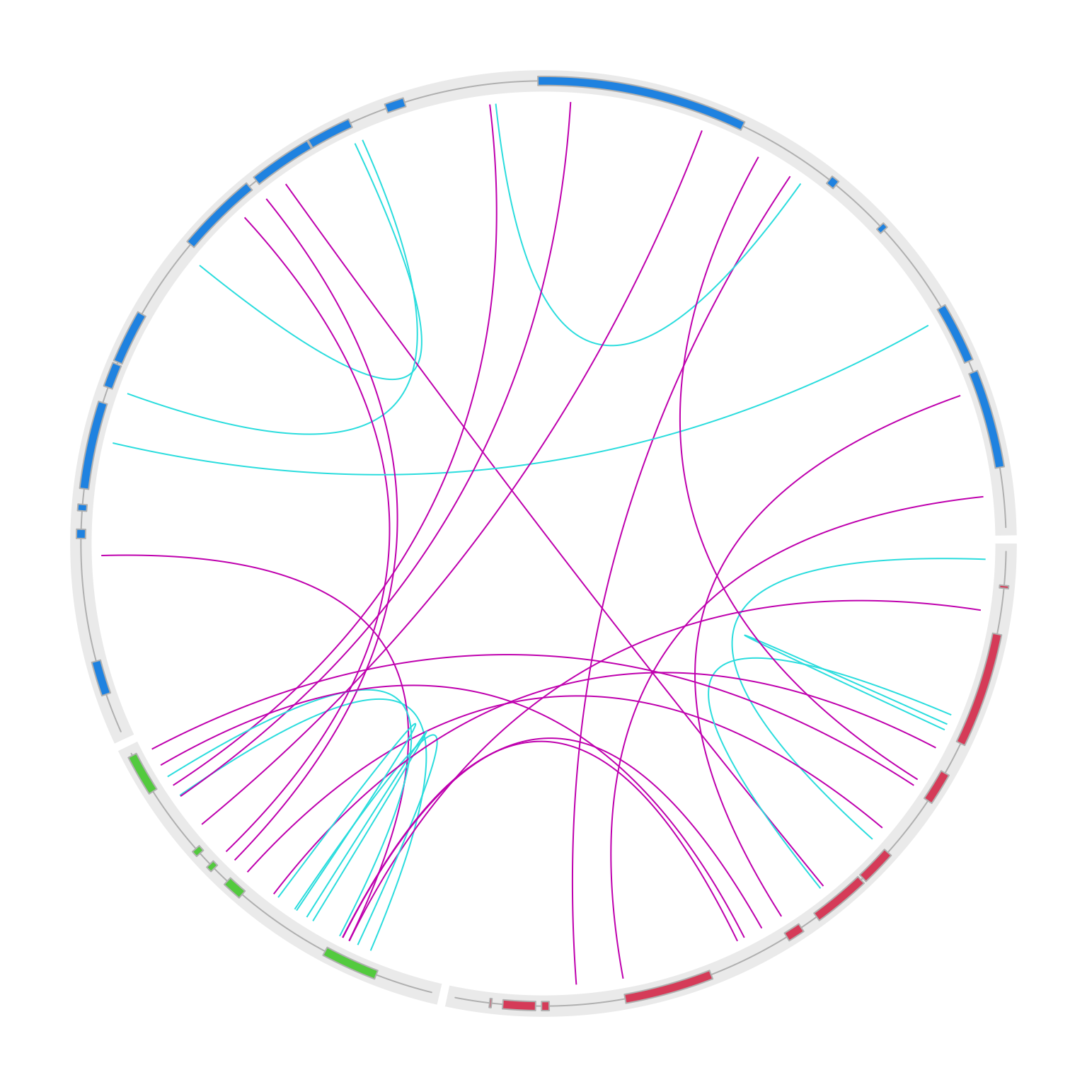
circos.clear()OK, it already looks good, but the intragenic and intergenic translocations are all put inside the circle, which makes it
a little bit difficult to differentiate. To move the intragenic translocations to the outside of the circle, we only need
to set argument h to a negative value, so that the link will be flipped onto the outside of the circle. Also note we need
to set rou which is the position of the link end. Here we set h to 1 which is the top border of the gene model track.
circos.initialize(c("A", "B", "C"), xlim = cbind(c(0, 0, 0), c(1, 0.5, 2)))

circos.track(ylim = c(0, 1), panel.fun = function(x, y) {
    tb = df[df[, 1] == CELL_META$sector.index, ]
    circos.lines(CELL_META$xlim, c(0.5, 0.5), col = "grey")
    circos.rect(tb[, 2], 0.1, tb[, 3], 0.9, col = 1+CELL_META$sector.numeric.index, border = "grey")
}, track.height = mm_h(4), bg.border = NA, bg.col = "#EEEEEE")

for(i in seq_len(nrow(link))) {
    if(link$gene1[i] == link$gene2[i]) {
        circos.link(link$gene1[i], link$x1[i], link$gene2[i], link$x2[i], col = 5, h = -0.1, rou = 1)
    } else {
        circos.link(link$gene1[i], link$x1[i], link$gene2[i], link$x2[i], col = 6)
    }
}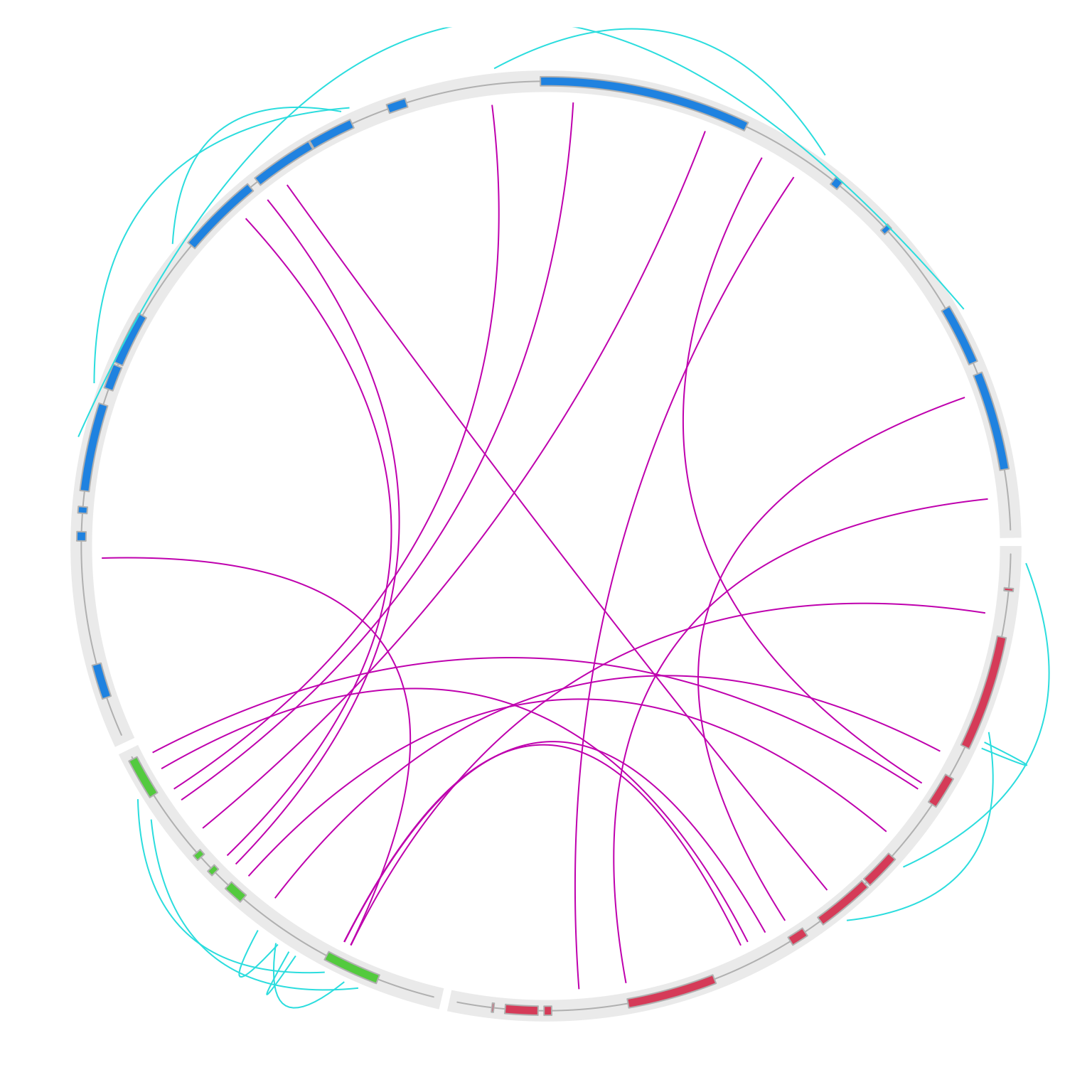
circos.clear()Now note since intergenic links are drawn outside of the circle, the outer space might not be enough. This can be easily
fixed by setting circos.par(circle.margin = ...) to increase the outer margin of the circular plot (the value is the proportion to the radius of the unit circle). I also increase the gap between two neighbouring genes to 10 degrees.
One last thing, when the two ends of the intragenic link are too far, the default link might be too sharp. Here
I also set w = 0.1 to make outside links “fat”.
circos.par(circle.margin = 0.1, gap.degree = 10)
circos.initialize(c("A", "B", "C"), xlim = cbind(c(0, 0, 0), c(1, 0.5, 2)))

circos.track(ylim = c(0, 1), panel.fun = function(x, y) {
    tb = df[df[, 1] == CELL_META$sector.index, ]
    circos.lines(CELL_META$xlim, c(0.5, 0.5), col = "grey")
    circos.rect(tb[, 2], 0.1, tb[, 3], 0.9, col = 1+CELL_META$sector.numeric.index, border = "grey")
}, track.height = mm_h(4), bg.border = NA, bg.col = "#EEEEEE")

for(i in seq_len(nrow(link))) {
    if(link$gene1[i] == link$gene2[i]) {
        circos.link(link$gene1[i], link$x1[i], link$gene2[i], link$x2[i], col = 5, h = -0.1, rou = 1, w = 0.1)
    } else {
        circos.link(link$gene1[i], link$x1[i], link$gene2[i], link$x2[i], col = 6)
    }
}
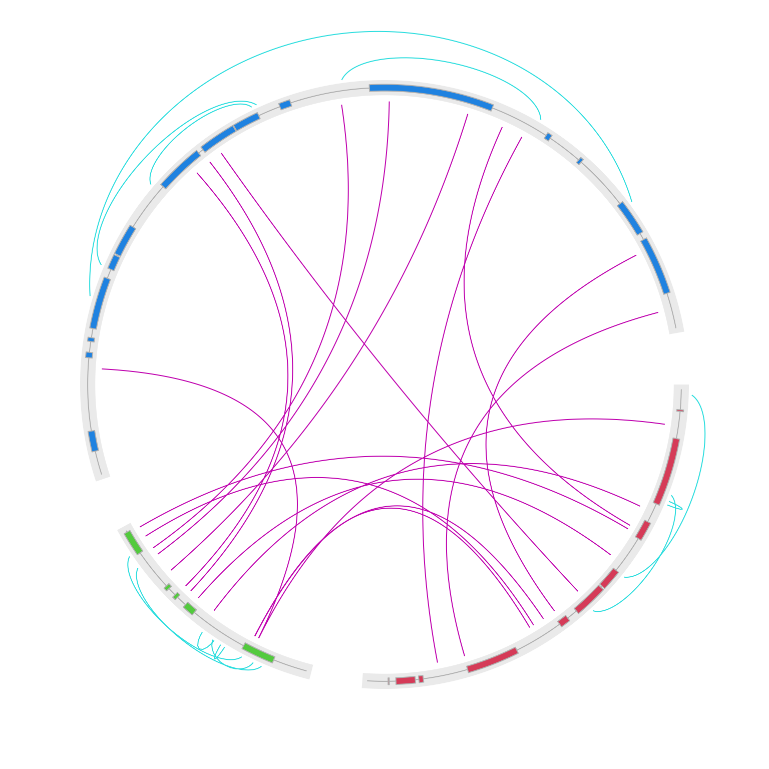
circos.clear()For the outside links, we may want the link to be shorter if its two ends are
closer to each other. We can dynamically calculate the value of h according
to the distance of a link’s two ends. Intuitively, we measure the distance by
the degree difference of the two ends on the circle.
We first write a simple function which returns h based on the degree difference.
in get_h(), if the degree difference is larger than 120 degrees, we let h take -0.15,
and if the degree difference is smaller than 20 degrees, we let h take -0.05.
get_h = function(degree_difference) {
    max_degree_difference = 120
    min_degree_difference = 20

    max_h = 0.15
    min_h = 0.05

    if(degree_difference >= max_degree_difference) {
        return(-max_h)
    }
    if(degree_difference <= min_degree_difference) {
        return(-min_h)
    }

    h = (degree_difference - min_degree_difference)/(max_degree_difference - min_degree_difference)*(max_h - min_h) + min_h
    -h
}
Next we write another function which calculates the degree difference. Note for simplicity, we only look at the link where
its two ends are in the same sector. In get_degree_difference(), get.cell.meta.data("cell.xlim", ...) is used to get
the data range on a specific sector, get.cell.meta.data("xplot", ...) is used to get the width of the sector measured by degree. Note since the data coordinates in sectors are always clockwise, xplot[1] is larger than xplot[2].
get_degree_difference = function(sector, x1, x2) {
    cell.xlim = get.cell.meta.data("cell.xlim", sector.index = sector, track.index = 1)
    xplot = get.cell.meta.data("xplot", sector.index = sector, track.index = 1)
    abs(x2 - x1)/(cell.xlim[2] - cell.xlim[1])*(xplot[1] - xplot[2])
}
With get_h() and get_degree_difference(), we can dynamically get the value of h
circos.par(circle.margin = 0.1, gap.degree = 10)
circos.initialize(c("A", "B", "C"), xlim = cbind(c(0, 0, 0), c(1, 0.5, 2)))

circos.track(ylim = c(0, 1), panel.fun = function(x, y) {
    tb = df[df[, 1] == CELL_META$sector.index, ]
    circos.lines(CELL_META$xlim, c(0.5, 0.5), col = "grey")
    circos.rect(tb[, 2], 0.1, tb[, 3], 0.9, col = 1+CELL_META$sector.numeric.index, border = "grey")
}, track.height = mm_h(4), bg.border = NA, bg.col = "#EEEEEE")

for(i in seq_len(nrow(link))) {
    if(link$gene1[i] == link$gene2[i]) {
        degree_difference = get_degree_difference(link$gene1[i], link$x1[i], link$x2[i])
        h = get_h(degree_difference)
        circos.link(link$gene1[i], link$x1[i], link$gene2[i], link$x2[i], col = 5, h = h, rou = 1, w = 0.1)
    } else {
        circos.link(link$gene1[i], link$x1[i], link$gene2[i], link$x2[i], col = 6)
    }
}
circos.clear()