In Web of Science, you can generate a nice citation map to show how your papers are cited world wide. In this blog post, I will demonstrate how to fetch the citation data and how to make such citation map in R.
The citation data is not straightforward to find. Since the citation map is presented on a web page, the data is actually downloaded by the browser. Thus, we just need to find the corresponding file there.
In the following steps, I assume you are using Chrome browser.
Step 1: Log into your personal Web of Science.
Step 2: Open the “Developer Tools”. There are two ways to open it.
- right click on the web page and click “Inspect” (which is the last one in the menu).
- or, in Chrome, View -> Developer -> Developer’s Tools
Step 3: In your Web of Science dashboard, click “My research profile”.

Step 4: In this page, click “Open dashboard” next to “Metrics”.
Step 5: Scroll downward to the section “Geographic Citation Map”, click “Click to show map”.

Step 6: In the Developer Tool, click on the “Netowrk” tab. You might see
there are many files under downloading. Once all the files are downloaded, double click on the file above
natigation_poin.svg (with name ?task_id=..., normally the one with the largest file size).

This will download the file, which is a json file that contains all the publication data for the citation map.

Step 7: Save the output into a file, e.g, by pressing “Ctrl + s”. Let’s save it into a file called citation.json.
Unfortunately, this json file cannot be directly read by packages such as jsonlite or rjson (Actually it is not in json format). We need to slightly modify it a little bit.
The content in citation.json is a valid JavaScript command. We explicitely let it be assgined to a variable. Simply add citation = in the very beginning
of citation.json (we assume the variable is called citation).

Step 8: Now we can use the V8 package to execute the JavaScript code.
library(V8)
ct = v8()
ct$source("~/citation.json")
## [1] "[object Object]"Step 9: Transfer the JavaScript variable citation into R by the get() method.
citation = ct$get("citation")OK, now the citation data is obtained, and we can process it in R.
I will not show the value of citation here because it is a little bit complex. I only take the results element which is a data frame.
Also I only take the first four columns and the fifth column in results contains all the paper information (e.g. authors, titles) which is not needed for the visualization.
results = citation$results[, 1:4]
head(results)
## address publicationCount lat lon
## 1 Putian, China 2 25.35331 119.05826
## 2 Blacksburg, United States 10 37.22957 -80.41394
## 3 Richmond, United States 7 37.55376 -77.46026
## 4 Toronto, Canada 328 43.64455 -79.40712
## 5 New Haven, United States 75 41.30815 -72.92816
## 6 Sydney, Australia 135 -33.86785 151.20732Now in the object results, there are the geographical coordinates (lat and lon), which can be used for the map.
The next chunk of code is optional. It basically merges different insitutes/universities in the same city into one record.
tb = data.frame(address = tapply(results$address, results$address, function(x) x[1]),
                publicationCount = tapply(results$publicationCount, results$address, sum),
                lat = tapply(results$lat, results$address, mean),
                lon = tapply(results$lon, results$address, mean))
Next we draw the world map. I basically follow a tutorial from the internet (https://r-spatial.org/r/2018/10/25/ggplot2-sf.html).
library("sf")
library("rnaturalearth")
library("rnaturalearthdata")
world = ne_countries(scale = "medium", returnclass = "sf")
library(ggplot2)
library(ggrepel)
library(RColorBrewer)
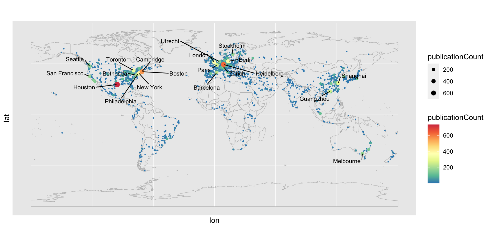
ggplot(data = world) + geom_sf(color = "grey", fill = NA) +
geom_point(data = tb[order(tb$publicationCount), ],
aes(x = lon, y = lat, color = publicationCount, size = publicationCount)) +
scale_colour_gradientn(colours = rev(brewer.pal(9, "Spectral"))) +
scale_size(range = c(0.2, 3)) +
geom_text_repel(data = tb[order(-tb$publicationCount)[1:20], ],
mapping = aes(x = lon, y = lat, label = gsub(", .*$", "", address)),
box.padding = 0.5, max.overlaps = Inf, min.segment.length = 0, size = 3)