Hierarchical clustering is a widely used approach for data analysis.
In this post, I will demonstrate the internal structure of a hclust object.
I first generate a random matrix and apply hclust().
set.seed(123456)
m = matrix(rnorm(25), 5)
rownames(m) = letters[1:5]
hc = hclust(dist(m))
Typing the hc object simply prints the basic information of the object.
hc##
## Call:
## hclust(d = dist(m))
##
## Cluster method : complete
## Distance : euclidean
## Number of objects: 5And plot() function draws the clustering results:
plot(hc)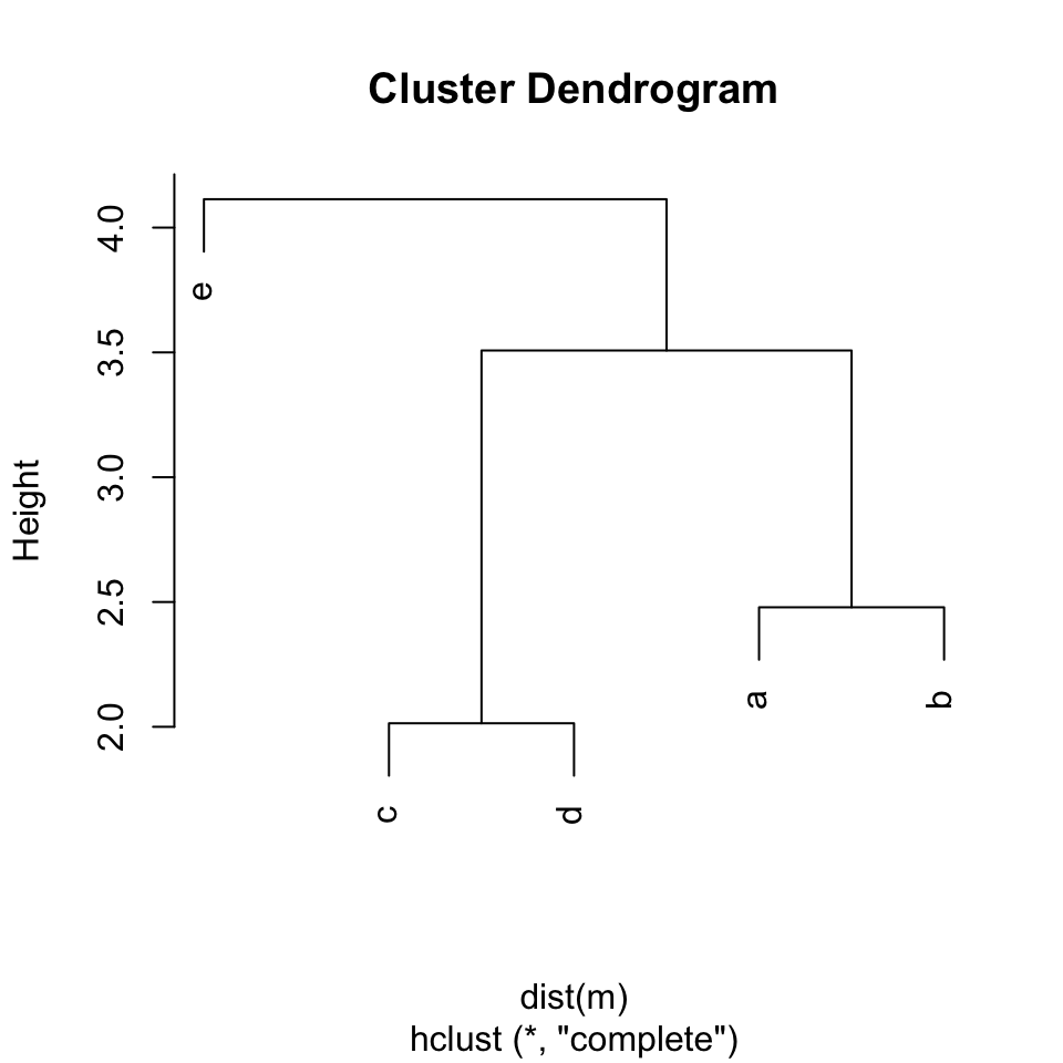
Now, what is hiding behind the hc object? Let’s first try str() function to reveal its internals:
str(hc)## List of 7
## $ merge : int [1:4, 1:2] -3 -1 1 -5 -4 -2 2 3
## $ height : num [1:4] 2.01 2.48 3.51 4.11
## $ order : int [1:5] 5 3 4 1 2
## $ labels : chr [1:5] "a" "b" "c" "d" ...
## $ method : chr "complete"
## $ call : language hclust(d = dist(m))
## $ dist.method: chr "euclidean"
## - attr(*, "class")= chr "hclust"So, hc is just a simple list with 7 elements. The last three ones method, call and dist.method
are less interesting because they are kind like label marks of the analysis. We will
look at the first four elements.
To correctly understand the hc object, we need to be careful with the orders of the vectors/matrices
in hc. We start with labels and order.
hc$labels## [1] "a" "b" "c" "d" "e"hc$order## [1] 5 3 4 1 2The labels element contains text labels of the items in their original orders. Here hc
is from a matrix m, so the order of labels corresponds to the original row order in the matrix.
The order in order is different from that in labels. As hierarchical clustering reorders
the items, order element contains results after the reordering. In the following order vector:
hc$order## [1] 5 3 4 1 2the first value means item 5 is in position 1 after reordering, item 3 is in position 2 after reordering, etc. So if mapping labels to order, it will be:
hc$labels[hc$order]## [1] "e" "c" "d" "a" "b"As you can see in the plot, after the reordering by hierarchical clustering, item “e” locates on the very left, and then item “c”, “d”, “a” and “b”.
Next let’s check the merge and height elements in the hc object:
hc$merge## [,1] [,2]
## [1,] -3 -4
## [2,] -1 -2
## [3,] 1 2
## [4,] -5 3hc$height## [1] 2.014138 2.478801 3.507676 4.113743On the first glance, it may look a little bit unnatural that there are both positive and negative
integers in merge. Actually, merge uses different signs to represent different types of objects in the
clustering, i.e. an item or a sub-cluster.
First we need to know, hclust() applies the agglomerative hierarchical clustering procedure, which is “bottom-up” approach, as shown in the following figures.
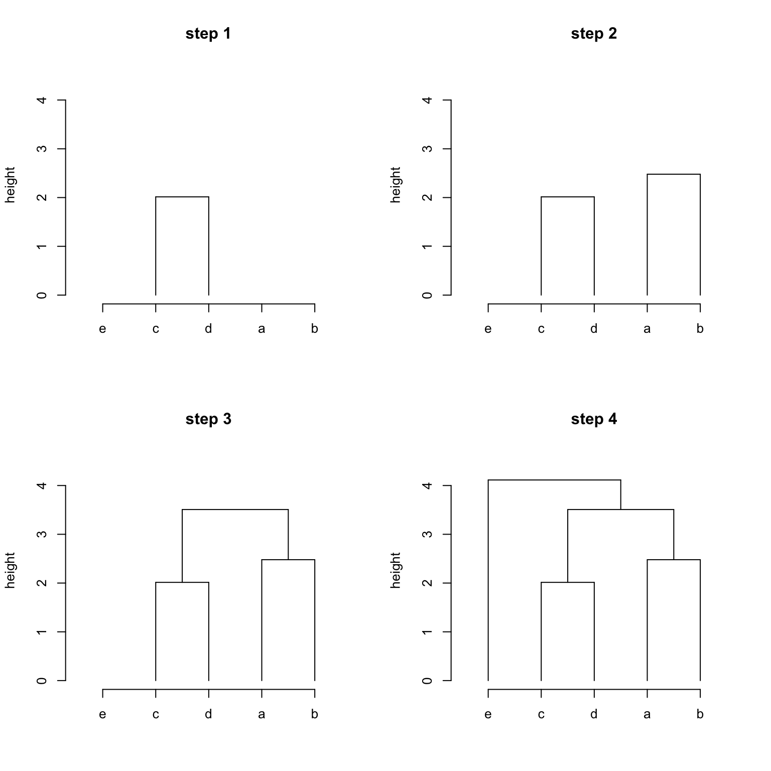
So merge records the steps of clustering where negative integers correspond to items (or leaves)
and positive integers correspond to intermediate sub-clusters. Then merge can be read as:
hc$merge## [,1] [,2]
## [1,] -3 -4
## [2,] -1 -2
## [3,] 1 2
## [4,] -5 3- Step 1 / row 1: item 3 (“c”) and 4 (“d”) are clustered. The sub-cluster has an index 1.
- Step 2 / row 2: item 1 (“a”) and 2 (“b”) are clustered. The sub-cluster has an index 2.
- Step 3 / row 3: Note now the values are both positive. This means sub-cluster 1 and sub-cluster 2 are merged where sub-cluster 1 was constructed in row 1 and sub-cluster 2 was constructed in row 2.
- Step 4 / row 4: This row contains both negative and positive values. This means a single item 5 (“e”) and a sub-cluster is merged where the sub-cluster is from row 3.
hc$height corresponds to hc$merge, and it is the height of each sub-cluster.
With all the elements in hc being explained, let’s try to draw the clustering. Let’s draw the clustering
according to the steps in hc$merge.
The first step is to cluster item 3 and item 4. We know the height of this sub-cluster is hc$height[1], but what is missing are the positions of items on x-axis, i.e. the horizontal positions of item 3 and 4. Let’s
try to get them.
We know the following are the reordered labels on the plot:
hc$labels[hc$order]## [1] "e" "c" "d" "a" "b"which locate at x = 1, 2, 3, 4, 5. However, it is not in the original order.
As in hc$merge, the “negative” integers correspond to the orignal order (e.g.
-2 means item 2), thus we need to know the positions of items where items are in
their original orders.
This can be done by mapping with the labels:
# 1:5 is the positions on x-axis
map = structure(1:5, names = hc$labels[hc$order])
# and we use the named vector to reorder into the original order
x = map[hc$labels]
x
## a b c d e
## 4 5 2 3 1Or we can directly use the following code which takes the order of hc$order.
x = order(hc$order)
x
## [1] 4 5 2 3 1In hc$order, values are the original indices of items, and the index of hc$order itself
is the positions on x-axis in the clustering plot.
hc$order
  value 5 3 4 1 2  # indices of items, i.e. item 5, item 3, ...
  pos   1 2 3 4 5  # pos in x-axis in the plot
If we apply order() on the vector hc$order which is 5 3 4 1 2, the first value
in the returned vector is the position of “1” (item 1) in 5 3 4 1 2 which is 4,
and the second value is the position of “2” (item 2) in 5 3 4 1 2 which is 5, etc.
This means, applying order() on hc$order returns a vector in the original order of items
and values are the positions on x-axis.
OK, now we can draw the clustering step-by-step.
Step 1 / row 1 in hc$merge: connects item 3 (“c”) and 4 (“d”):
plot(NULL, xlim = c(0.5, 5.5), ylim = c(0, max(hc$height)*1.1), axes = FALSE, ann = FALSE)
axis(side = 1, at = 1:5, labels = hc$labels[hc$order])
axis(side = 2)

# the first row in `merge` is '[1,]   -3   -4'
segments(x[3], hc$height[1], x[4], hc$height[1])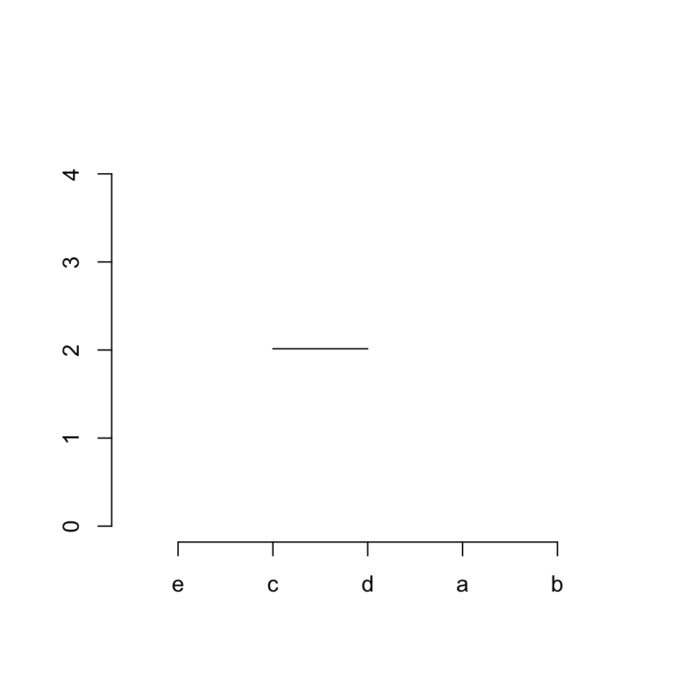
Step 2 / row 2: connects item 1 (“a”) and 2 (“b”):
plot(NULL, xlim = c(0.5, 5.5), ylim = c(0, max(hc$height)*1.1), axes = FALSE, ann = FALSE)
axis(side = 1, at = 1:5, labels = hc$labels[hc$order])
axis(side = 2)

segments(x[3], hc$height[1], x[4], hc$height[1])
# the second row in `merge` is '[2,]   -1   -2'
segments(x[1], hc$height[2], x[2], hc$height[2])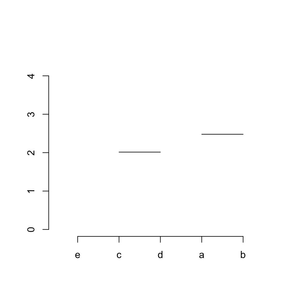
Step 3 / row 3: connects sub-cluster 1 and sub-cluster 2. Now there is a new thing. Since we are now connecting two sub-clusters, we need to connect to the “middle points” of the two sub-clusters. This can be done very easily. The middle point of sub-cluster 1 is the middle of item 3 between 4, and the middle point of sub-cluster 2 is the middle of item 1 between 2.
plot(NULL, xlim = c(0.5, 5.5), ylim = c(0, max(hc$height)*1.1), axes = FALSE, ann = FALSE)
axis(side = 1, at = 1:5, labels = hc$labels[hc$order])
axis(side = 2)

segments(x[3], hc$height[1], x[4], hc$height[1])
segments(x[1], hc$height[2], x[2], hc$height[2])

midpoint = numeric(0)
midpoint[1] = (x[3]+x[4])/2
midpoint[2] = (x[1]+x[2])/2

# the third row in `merge` is '[3,]    1    2'
segments(midpoint[1], hc$height[3], midpoint[2], hc$height[3])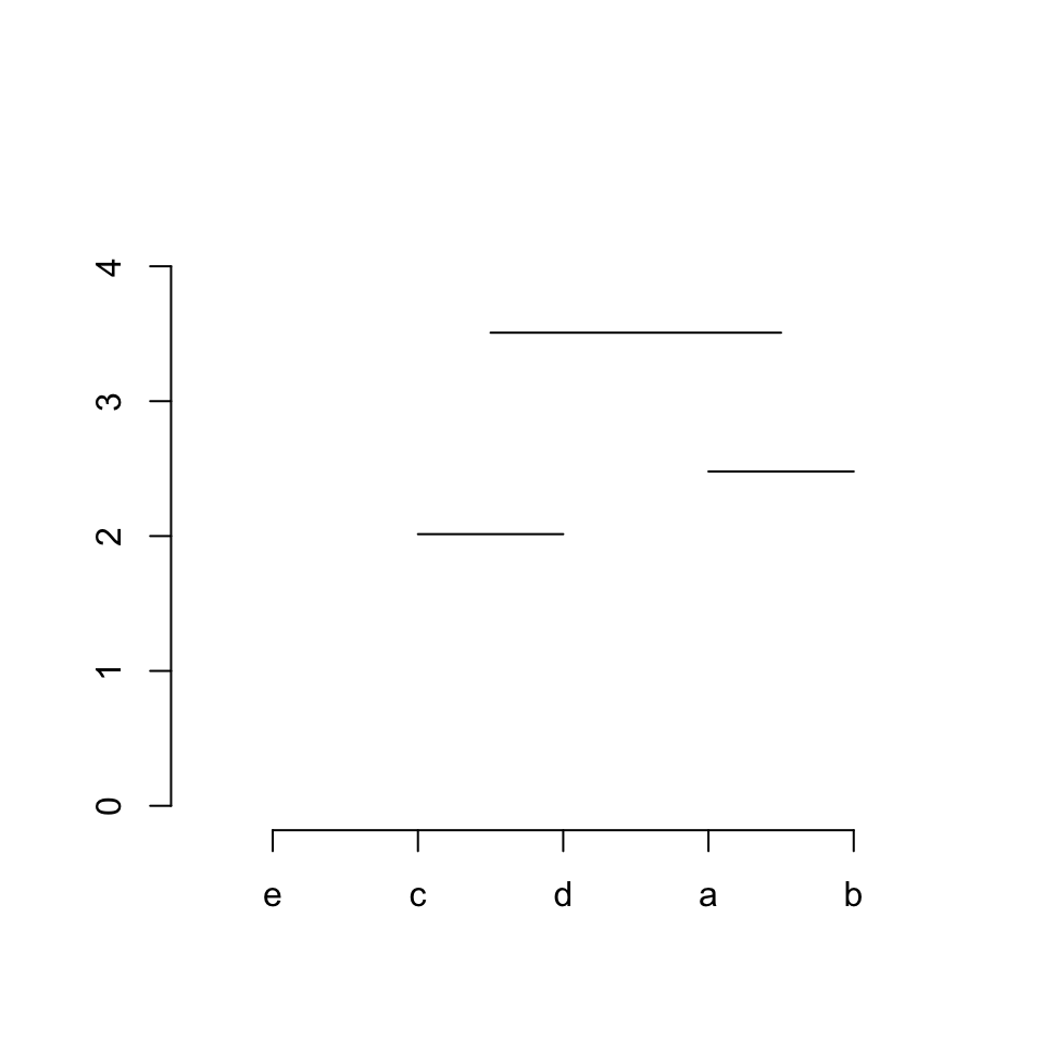
Step 4 / row 4: connects item 5 (“e”) and sub-cluster 3. Similarly, middle point of sub-cluster 3 needs to be calculated in advance which is the middle of the middle points of its two sub clusters (sub-cluster 1 and 2).
plot(NULL, xlim = c(0.5, 5.5), ylim = c(0, max(hc$height)*1.1), axes = FALSE, ann = FALSE)
axis(side = 1, at = 1:5, labels = hc$labels[hc$order])
axis(side = 2)

segments(x[3], hc$height[1], x[4], hc$height[1])
segments(x[1], hc$height[2], x[2], hc$height[2])

midpoint = numeric(0)
midpoint[1] = (x[3]+x[4])/2
midpoint[2] = (x[1]+x[2])/2

segments(midpoint[1], hc$height[3], midpoint[2], hc$height[3])

midpoint[3] = (midpoint[1] + midpoint[2])/2
# the third row in `merge` is '[4,]   -5    3'
segments(x[5], hc$height[4], midpoint[3], hc$height[4])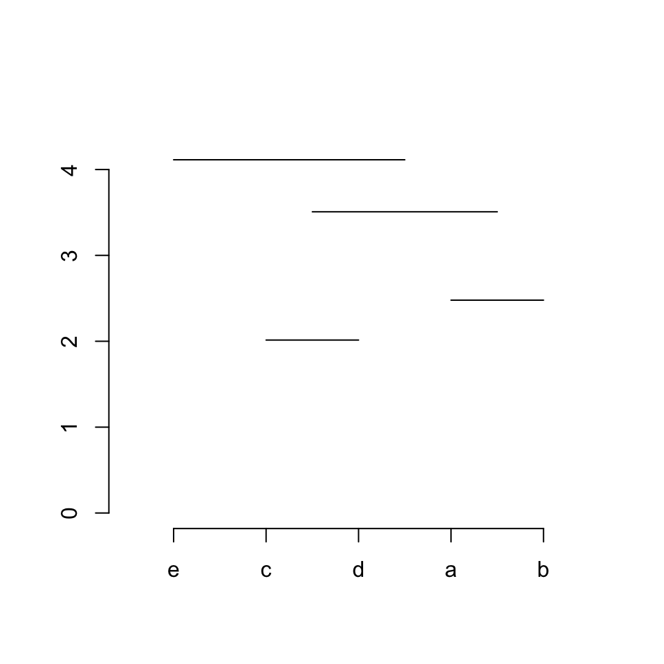
Vertical lines can be added as:
plot(NULL, xlim = c(0.5, 5.5), ylim = c(0, max(hc$height)*1.1), axes = FALSE, ann = FALSE)
axis(side = 1, at = 1:5, labels = hc$labels[hc$order])
axis(side = 2)

segments(x[3], hc$height[1], x[4], hc$height[1])
segments(x[3], 0, x[3], hc$height[1])
segments(x[4], 0, x[4], hc$height[1])

segments(x[1], hc$height[2], x[2], hc$height[2])
segments(x[1], 0, x[1], hc$height[2])
segments(x[2], 0, x[2], hc$height[2])

midpoint = numeric(0)
midpoint[1] = (x[3]+x[4])/2
midpoint[2] = (x[1]+x[2])/2

segments(midpoint[1], hc$height[3], midpoint[2], hc$height[3])
segments(midpoint[1], hc$height[3], midpoint[1], hc$height[1])
segments(midpoint[2], hc$height[3], midpoint[2], hc$height[2])

midpoint[3] = (midpoint[1] + midpoint[2])/2
segments(x[5], hc$height[4], midpoint[3], hc$height[4])
segments(midpoint[3], hc$height[4], midpoint[3], hc$height[3])
segments(x[5], 0, x[5], hc$height[4])
We can merge all these processes into a function. The function is quite
straightforward to understand. There are four if-else blocks which deal with:
- both children are leaves,
- left child is a leaf, right child is a sub-cluster,
- left child is a sub-cluster, right child is a leaf,
- both children are sub-clusters.
plot_hc = function(hc) {
    x = order(hc$order)
    nobs = length(x)

    if(length(hc$labels) == 0) {
        hc$labels = as.character(seq_along(hc$order))
    }

    plot(NULL, xlim = c(0.5, nobs + 0.5), ylim = c(0, max(hc$height)*1.1), axes = FALSE, ann = FALSE)
    axis(side = 1, at = 1:nobs, labels = hc$labels[hc$order])
    axis(side = 2)

    merge = hc$merge
    order = hc$order
    nr = nrow(merge)
    midpoint = numeric(nr)

    for(i in seq_len(nr)) {
        child1 = merge[i, 1]
        child2 = merge[i, 2]

        if(child1 < 0 && child2 < 0) { # both are leaves
            segments(x[ -child1 ],
                     hc$height[i],
                     x[ -child2 ],
                     hc$height[i])
            midpoint[i] = (x[ -child1 ] + x[ -child2 ])/2
            segments(x[ -child1 ], hc$height[i], x[ -child1 ], 0)
            segments(x[ -child2 ], hc$height[i], x[ -child2 ], 0)
        } else if(child1 < 0 && child2 > 0) {
            segments(x[ -child1 ],
                     hc$height[i],
                     midpoint[ child2 ],
                     hc$height[i])
            midpoint[i] = (x[ -child1 ] + midpoint[ child2 ])/2
            segments(x[ -child1 ], hc$height[i], x[ -child1 ], 0)
            segments(midpoint[ child2 ], hc$height[i], midpoint[ child2 ], hc$height[ child2 ])
        } else if(merge[i, 1] > 0 && merge[i, 2] < 0) {
            segments(midpoint[ child1 ],
                     hc$height[i],
                     x[ -child2 ],
                     hc$height[i])
            midpoint[i] = (midpoint[ child1 ] + x[ -child2 ])/2
            segments(midpoint[ child1 ], hc$height[i], midpoint[ child1 ], hc$height[ child1 ])
            segments(x[ -child2 ], hc$height[i], x[ -child2 ], 0)
        } else {
            segments(midpoint[ child1 ],
                     hc$height[i],
                     midpoint[ child2 ],
                     hc$height[i])
            midpoint[i] = (midpoint[ child1 ] + midpoint[ child2 ])/2
            segments(midpoint[ child1 ], hc$height[i], midpoint[ child1 ], hc$height[ child1 ])
            segments(midpoint[ child2 ], hc$height[i], midpoint[ child2 ], hc$height[ child2 ])
        }
    }
}
plot_hc(hc)
Let’s try a larger clustering object:
m2 = matrix(rnorm(1000), nrow = 100)
hc2 = hclust(dist(m2))
plot_hc(hc2)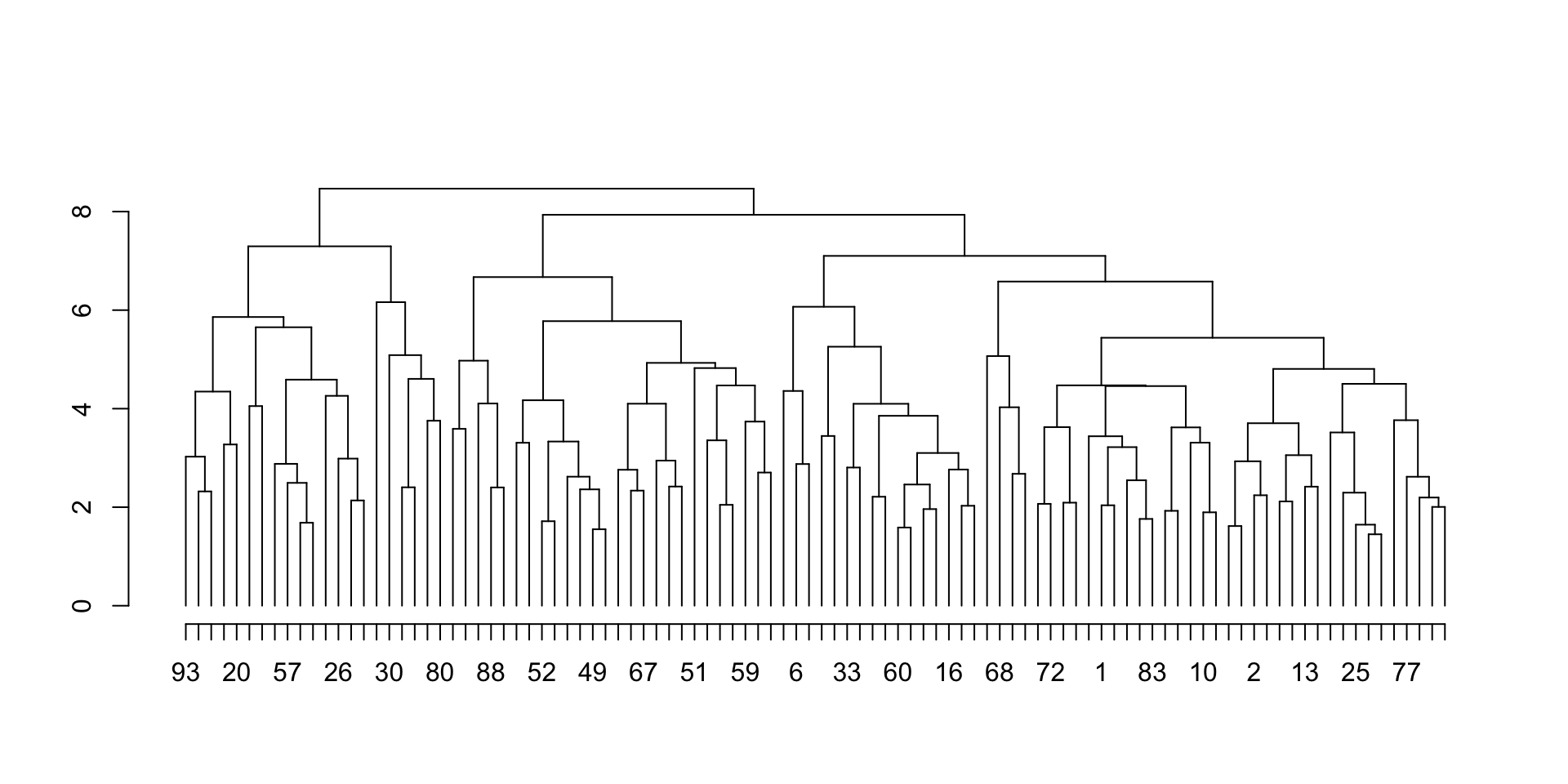
Connecting a parent node and two children nodes in the clustering graph can be generalized as: with
three points: (left_x, left_y), (top_x, top_y) and (right_x, right_y) which correspond to
xy coordinates of the left child, parent and right child, we can define a function to draw lines to connect
the three points.
The default connection actually connects the following points:
x-coordinates: left_x, left_x, right_x, right_x
y-coordinates: left_y, top_y, top_y, right_y
In plot_hc(), let’s abstract the code which draws connections between parent and children nodes to
parent_children_connections() which accepts coordinates of the three points.
plot_hc = function(hc) {
    x = order(hc$order)
    nobs = length(x)

    if(length(hc$labels) == 0) {
        hc$labels = as.character(seq_along(hc$order))
    }

    plot(NULL, xlim = c(0.5, nobs + 0.5), ylim = c(0, max(hc$height)*1.1), axes = FALSE, ann = FALSE)
    axis(side = 1, at = 1:nobs, labels = hc$labels[hc$order])
    axis(side = 2)

    merge = hc$merge
    order = hc$order
    height = hc$height
    nr = nrow(merge)
    midpoint = numeric(nr)

    for(i in seq_len(nr)) {
        child1 = merge[i, 1]
        child2 = merge[i, 2]

        if(child1 < 0 && child2 < 0) { # both are leaves
            midpoint[i] = (x[ -child1 ] + x[ -child2 ])/2
            parent_children_connections(
                x[-child1], 0,
                midpoint[i], height[i],
                x[-child2], 0
            )
        } else if(child1 < 0 && child2 > 0) {
            midpoint[i] = (x[ -child1 ] + midpoint[ child2 ])/2
            parent_children_connections(
                x[-child1], 0,
                midpoint[i], height[i],
                midpoint[child2], height[child2]
            )
        } else if(child1 > 0 && child2 < 0) {
            midpoint[i] = (midpoint[ child1 ] + x[ -child2 ])/2
            parent_children_connections(
                midpoint[child1], height[child1],
                midpoint[i], height[i],
                x[-child2], 0
            )
        } else {
            midpoint[i] = (midpoint[ child1 ] + midpoint[ child2 ])/2
            parent_children_connections(
                midpoint[child1], height[child1],
                midpoint[i], height[i],
                midpoint[child2], height[child2]
            )
        }
    }
}
The following function is the default way to connect parent and children nodes:
parent_children_connections = function(left_x, left_y, top_x, top_y, right_x, right_y) {
    lines(c(left_x, left_x, right_x, right_x),
          c(left_y, top_y, top_y, right_y))
}
plot_hc(hc)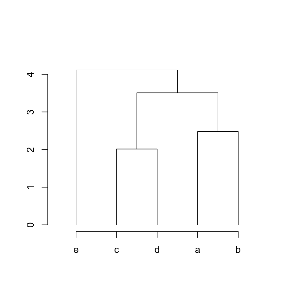
We can define a new way as:
x-coordinates: left_x, top_x, right_x
y-coordinates: left_y, top_y, right_y
parent_children_connections = function(left_x, left_y, top_x, top_y, right_x, right_y) {
lines(c(left_x, top_x, right_x),
c(left_y, top_y, right_y))
}
plot_hc(hc)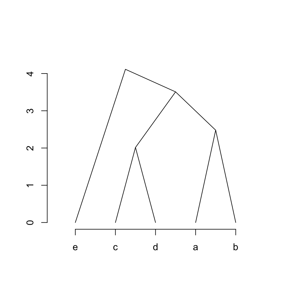
Hierarchical clustering constructs a binary tree, where a parent always has two children in the tree. In the next post, I will introduce a more general structure, the dendrogram.