Suppl 3. Compare online and local GREAT
Zuguang Gu ( z.gu@dkfz.de )
2024-02-27
Source:vignettes/suppl_compare_online_and_local.Rmd
suppl_compare_online_and_local.RmdIn this document, we will compare the enrichment results from online GREAT and local GREAT. The four datasets are all from UCSC table browser. Parameters are:
clade = Mammal
genome = Human
assembly = GRCh37/hg19
group = Regulation
track = ENCODE 3 TFBS
table: A549 JUN, A549 ELF1, H1-hESC RXRA, GM12878 MYB
And in the “Retrieve and display data” section:
output format = BED - browser extensible dataThen click the button “get output”.
We first read the files into GRanges objects:
read_bed = function(f) {
    df = read.table(f)
    df = df[df[, 1] %in% paste0("chr", c(1:22, "X", "Y")), ]
    GRanges(seqnames = df[, 1], ranges = IRanges(df[, 2] + 1, df[, 3]))
}
grl = list()
grl$A549_JUN = read_bed("data/tb_encTfChipPkENCFF708LCH_A549_JUN_hg19.bed")
grl$A549_ELF1 = read_bed("data/tb_encTfChipPkENCFF533NIV_A549_ELF1_hg19.bed")
grl$H1_hESC_RXRA = read_bed("data/tb_encTfChipPkENCFF369JAI_H1_hESC_RXRA_hg19.bed")
grl$GM12878_MYB = read_bed("data/tb_encTfChipPkENCFF215YWS_GM12878_MYB_hg19.bed")
sapply(grl, length)
## A549_JUN A549_ELF1 H1_hESC_RXRA GM12878_MYB
## 1726 11577 2092 3748A549_JUN (1726 input regions)
Apply both online and local GREAT analysis. Note online GREAT exclude gap regions, and in local GREAT, by default gap regions are removed as well.
gr = grl$A549_JUN
job = submitGreatJob(gr)
tbl = getEnrichmentTables(job)
tb1 = tbl[["GO Biological Process"]]

res = great(gr, "GO:BP", "hg19")
tb2 = getEnrichmentTable(res)
tb1 and tb2 contain the full table of all GO terms under test. First we take the common GO terms in the two result tables.
## [1] 4578The significant GO terms from the two tables.
lt2 = list(online = tb1$ID[tb1$Binom_Adjp_BH < 0.001],
          local = tb2$id[tb2$p_adjust < 0.001])
plot(euler(lt2), quantities = TRUE, main = "A549_JUN")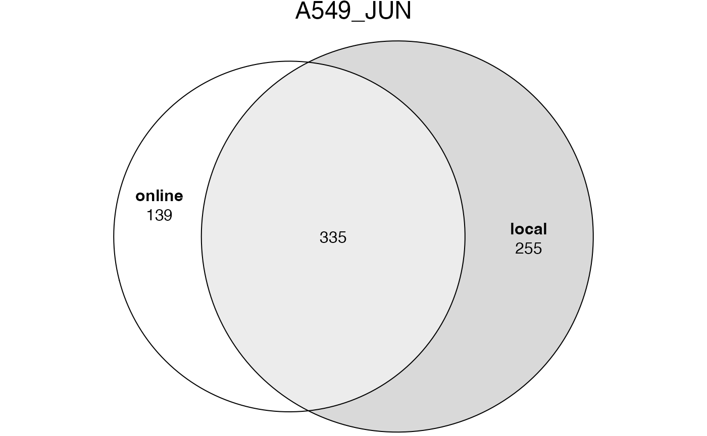
Next we compare the observed region hits and fold enrichment in the two results.
par(mfrow = c(1, 2))
plot(tb1$Binom_Observed_Region_Hits, tb2$observed_region_hits, pch = 16, col = "#00000010",
    xlab = "online GREAT", ylab = "local GREAT", main = "Observed region hits")
plot(tb1$Binom_Fold_Enrichment, tb2$fold_enrichment, pch = 16, col = "#00000010",
    xlab = "online GREAT", ylab = "local GREAT", main = "Fold enrichment")
Next we compare the two significant GO term lists by clustering them into groups.
lt3 = list(online = data.frame(id = tb1$ID, p_adjust = tb1$Binom_Adjp_BH),
           local = data.frame(id = tb2$id, p_adjust = tb2$p_adjust))
library(simplifyEnrichment)
se_opt$verbose = FALSE
simplifyGOFromMultipleLists(lt3, padj_cutoff = 0.001)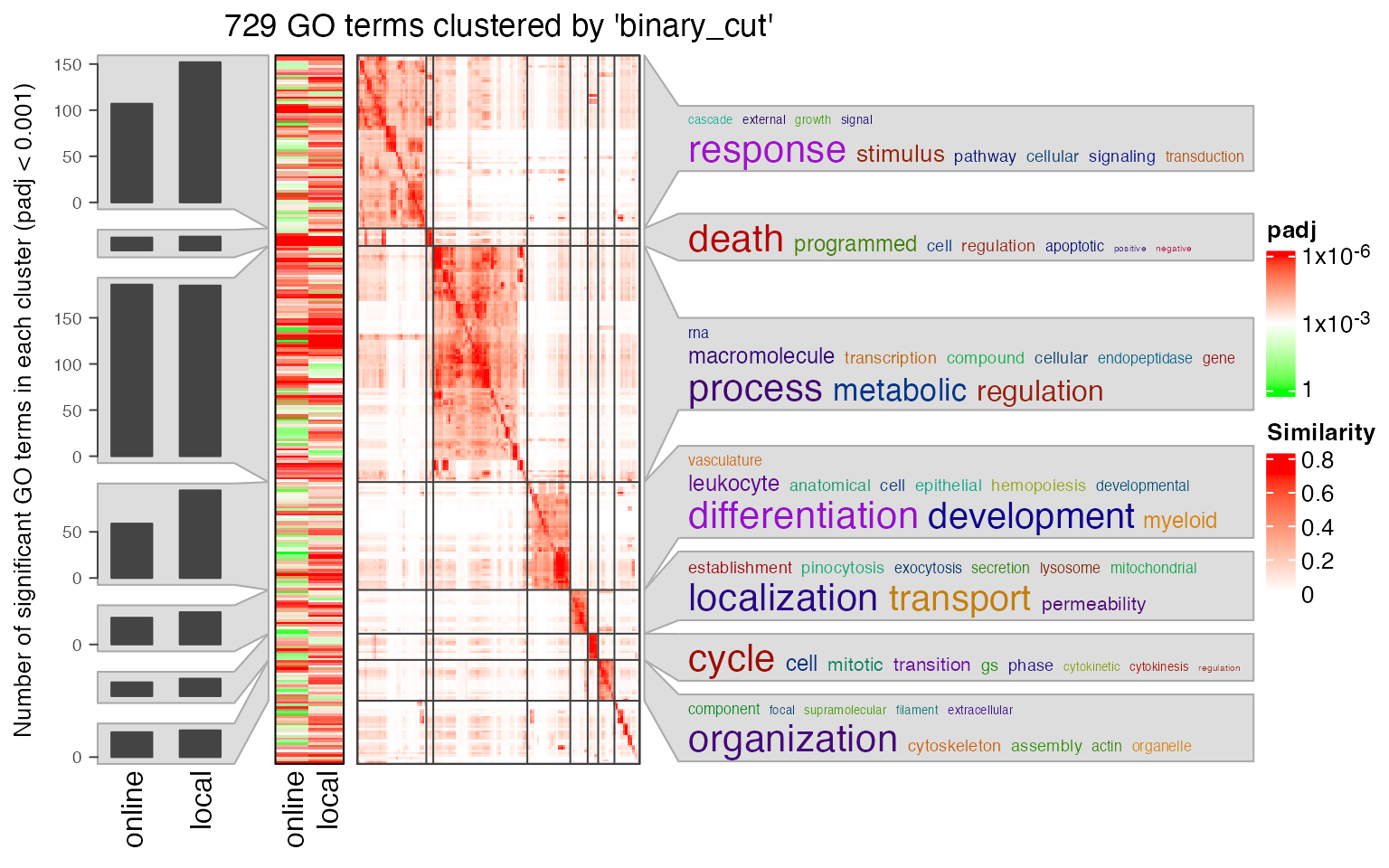
A549_ELF1 (11577 input regions)
Apply both online and local GREAT analysis:
gr = grl$A549_ELF1
job = submitGreatJob(gr)
tbl = getEnrichmentTables(job)
tb1 = tbl[["GO Biological Process"]]

res = great(gr, "GO:BP", "hg19")
tb2 = getEnrichmentTable(res)
tb1 and tb2 contain the full table of all GO terms under test. First we take the common GO terms in the two result tables.
## [1] 7552The significant GO terms from the two tables.
lt2 = list(online = tb1$ID[tb1$Binom_Adjp_BH < 0.001],
          local = tb2$id[tb2$p_adjust < 0.001])
plot(euler(lt2), quantities = TRUE, main = "A549_ELF1")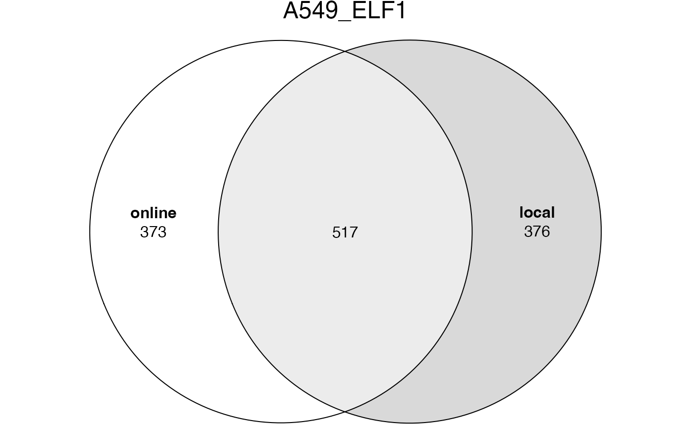
Next we compare the observed region hits and fold enrichment in the two results.
par(mfrow = c(1, 2))
plot(tb1$Binom_Observed_Region_Hits, tb2$observed_region_hits, pch = 16, col = "#00000010",
    xlab = "online GREAT", ylab = "local GREAT", main = "Observed region hits")
plot(tb1$Binom_Fold_Enrichment, tb2$fold_enrichment, pch = 16, col = "#00000010",
    xlab = "online GREAT", ylab = "local GREAT", main = "Fold enrichment")
Next we compare the two significant GO term lists by clustering them into groups.
lt3 = list(online = data.frame(id = tb1$ID, p_adjust = tb1$Binom_Adjp_BH),
           local = data.frame(id = tb2$id, p_adjust = tb2$p_adjust))
library(simplifyEnrichment)
se_opt$verbose = FALSE
simplifyGOFromMultipleLists(lt3, padj_cutoff = 0.001)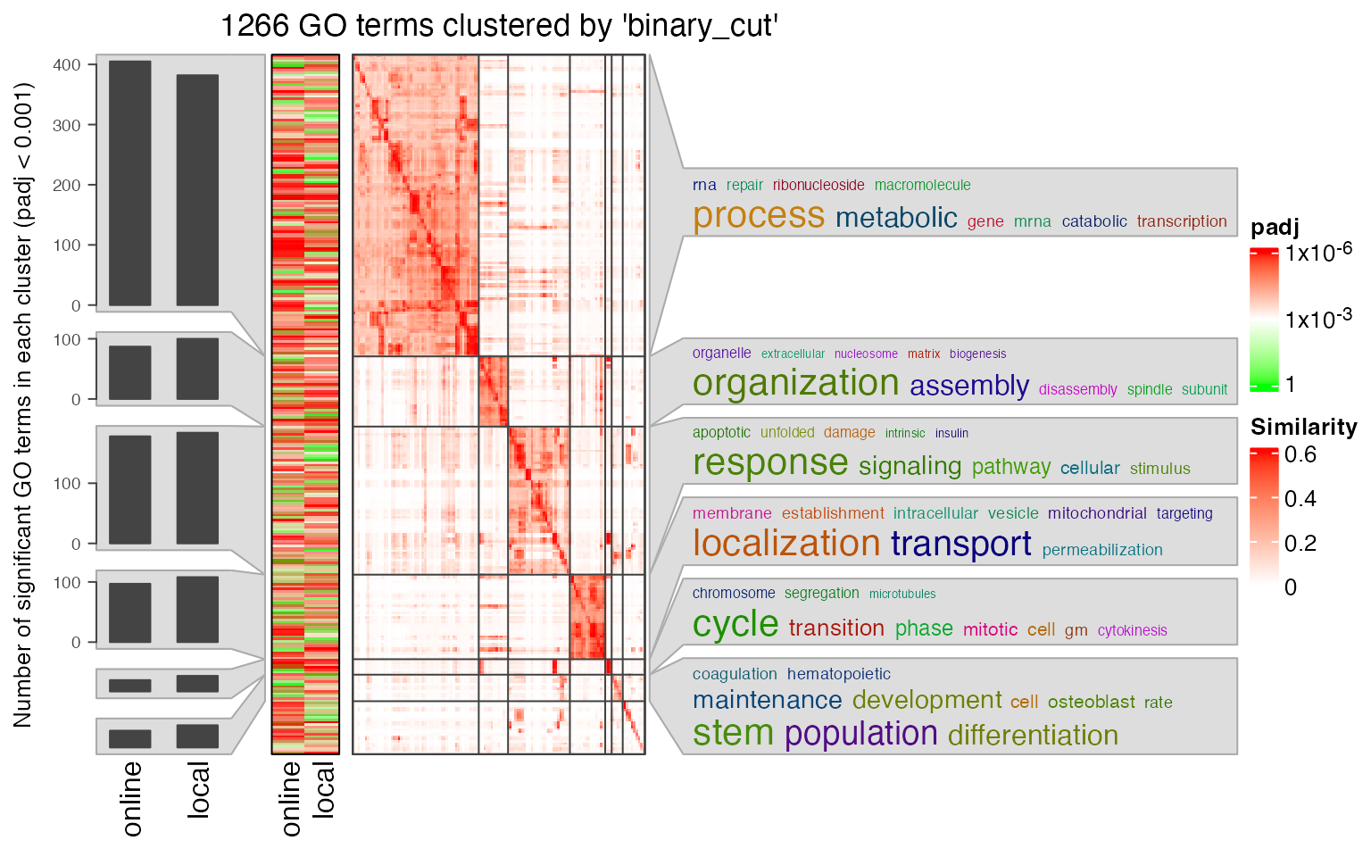
H1_hESC_RXRA (2092 input regions)
Apply both online and local GREAT analysis:
gr = grl$H1_hESC_RXRA
job = submitGreatJob(gr)
tbl = getEnrichmentTables(job)
tb1 = tbl[["GO Biological Process"]]

res = great(gr, "GO:BP", "hg19")
tb2 = getEnrichmentTable(res)
tb1 and tb2 contain the full table of all GO terms under test. First we take the common GO terms in the two result tables.
## [1] 4694The significant GO terms from the two tables.
lt2 = list(online = tb1$ID[tb1$Binom_Adjp_BH < 0.001],
          local = tb2$id[tb2$p_adjust < 0.001])
plot(euler(lt2), quantities = TRUE, main = "H1_hESC_RXRA")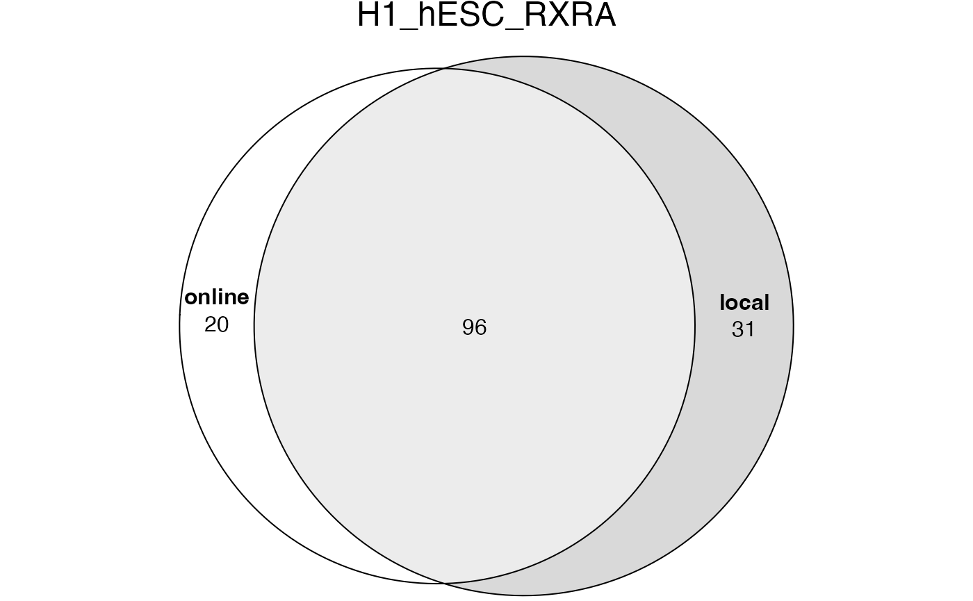
Next we compare the observed region hits and fold enrichment in the two results.
par(mfrow = c(1, 2))
plot(tb1$Binom_Observed_Region_Hits, tb2$observed_region_hits, pch = 16, col = "#00000010",
    xlab = "online GREAT", ylab = "local GREAT", main = "Observed region hits")
plot(tb1$Binom_Fold_Enrichment, tb2$fold_enrichment, pch = 16, col = "#00000010",
    xlab = "online GREAT", ylab = "local GREAT", main = "Fold enrichment")
Next we compare the two significant GO term lists by clustering them into groups.
lt3 = list(online = data.frame(id = tb1$ID, p_adjust = tb1$Binom_Adjp_BH),
           local = data.frame(id = tb2$id, p_adjust = tb2$p_adjust))
library(simplifyEnrichment)
se_opt$verbose = FALSE
simplifyGOFromMultipleLists(lt3, padj_cutoff = 0.001)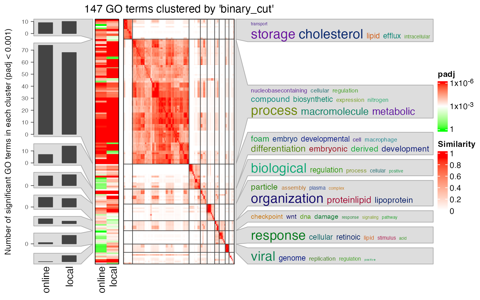
GM12878_MYB (3748 input regions)
Apply both online and local GREAT analysis:
gr = grl$GM12878_MYB
job = submitGreatJob(gr)
tbl = getEnrichmentTables(job)
tb1 = tbl[["GO Biological Process"]]

res = great(gr, "GO:BP", "hg19")
tb2 = getEnrichmentTable(res)
tb1 and tb2 contain the full table of all GO terms under test. First we take the common GO terms in the two result tables.
## [1] 5775The significant GO terms from the two tables.
lt2 = list(online = tb1$ID[tb1$Binom_Adjp_BH < 0.001],
          local = tb2$id[tb2$p_adjust < 0.001])
plot(euler(lt2), quantities = TRUE, main = "GM12878_MYB")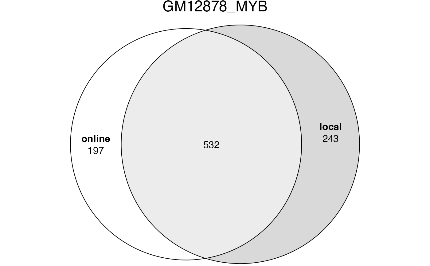
Next we compare the observed region hits and fold enrichment in the two results.
par(mfrow = c(1, 2))
plot(tb1$Binom_Observed_Region_Hits, tb2$observed_region_hits, pch = 16, col = "#00000010",
    xlab = "online GREAT", ylab = "local GREAT", main = "Observed region hits")
plot(tb1$Binom_Fold_Enrichment, tb2$fold_enrichment, pch = 16, col = "#00000010",
    xlab = "online GREAT", ylab = "local GREAT", main = "Fold enrichment")
Next we compare the two significant GO term lists by clustering them into groups.
lt3 = list(online = data.frame(id = tb1$ID, p_adjust = tb1$Binom_Adjp_BH),
           local = data.frame(id = tb2$id, p_adjust = tb2$p_adjust))
library(simplifyEnrichment)
se_opt$verbose = FALSE
simplifyGOFromMultipleLists(lt3, padj_cutoff = 0.001)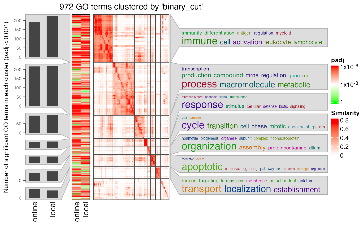
Session info
## R version 4.3.1 (2023-06-16)
## Platform: x86_64-apple-darwin20 (64-bit)
## Running under: macOS Ventura 13.2.1
##
## Matrix products: default
## BLAS:   /Library/Frameworks/R.framework/Versions/4.3-x86_64/Resources/lib/libRblas.0.dylib
## LAPACK: /Library/Frameworks/R.framework/Versions/4.3-x86_64/Resources/lib/libRlapack.dylib;  LAPACK version 3.11.0
##
## locale:
## [1] C/UTF-8/C/C/C/C
##
## time zone: Europe/Berlin
## tzcode source: internal
##
## attached base packages:
## [1] grid      stats4    stats     graphics  grDevices utils     datasets
## [8] methods   base
##
## other attached packages:
## [1] simplifyEnrichment_1.11.1 eulerr_7.0.0
## [3] rGREAT_2.5.4              GenomicRanges_1.52.1
## [5] GenomeInfoDb_1.36.4       IRanges_2.36.0
## [7] S4Vectors_0.40.2          BiocGenerics_0.48.1
## [9] knitr_1.44
##
## loaded via a namespace (and not attached):
##   [1] RColorBrewer_1.1-3
##   [2] jsonlite_1.8.8
##   [3] shape_1.4.6
##   [4] magrittr_2.0.3
##   [5] magick_2.8.0
##   [6] GenomicFeatures_1.52.2
##   [7] rmarkdown_2.25
##   [8] GlobalOptions_0.1.2
##   [9] fs_1.6.3
##  [10] BiocIO_1.10.0
##  [11] zlibbioc_1.46.0
##  [12] ragg_1.2.6
##  [13] vctrs_0.6.4
##  [14] Cairo_1.6-2
##  [15] memoise_2.0.1
##  [16] Rsamtools_2.16.0
##  [17] RCurl_1.98-1.12
##  [18] htmltools_0.5.7
##  [19] S4Arrays_1.0.6
##  [20] TxDb.Hsapiens.UCSC.hg19.knownGene_3.2.2
##  [21] progress_1.2.2
##  [22] curl_5.1.0
##  [23] sass_0.4.8
##  [24] bslib_0.6.1
##  [25] htmlwidgets_1.6.2
##  [26] desc_1.4.2
##  [27] cachem_1.0.8
##  [28] commonmark_1.9.0
##  [29] GenomicAlignments_1.36.0
##  [30] mime_0.12
##  [31] lifecycle_1.0.4
##  [32] iterators_1.0.14
##  [33] pkgconfig_2.0.3
##  [34] Matrix_1.6-1.1
##  [35] R6_2.5.1
##  [36] fastmap_1.1.1
##  [37] GenomeInfoDbData_1.2.10
##  [38] MatrixGenerics_1.12.3
##  [39] shiny_1.8.0
##  [40] clue_0.3-65
##  [41] digest_0.6.33
##  [42] colorspace_2.1-0
##  [43] AnnotationDbi_1.62.2
##  [44] rprojroot_2.0.3
##  [45] textshaping_0.3.7
##  [46] RSQLite_2.3.1
##  [47] org.Hs.eg.db_3.17.0
##  [48] filelock_1.0.2
##  [49] fansi_1.0.5
##  [50] httr_1.4.7
##  [51] polyclip_1.10-6
##  [52] abind_1.4-5
##  [53] compiler_4.3.1
##  [54] bit64_4.0.5
##  [55] doParallel_1.0.17
##  [56] BiocParallel_1.34.2
##  [57] DBI_1.1.3
##  [58] biomaRt_2.56.1
##  [59] rappdirs_0.3.3
##  [60] proxyC_0.3.3
##  [61] DelayedArray_0.26.7
##  [62] rjson_0.2.21
##  [63] tools_4.3.1
##  [64] httpuv_1.6.13
##  [65] glue_1.6.2
##  [66] restfulr_0.0.15
##  [67] GOSemSim_2.26.1
##  [68] promises_1.2.1
##  [69] gridtext_0.1.5
##  [70] polylabelr_0.2.0
##  [71] cluster_2.1.4
##  [72] generics_0.1.3
##  [73] hms_1.1.3
##  [74] xml2_1.3.6
##  [75] utf8_1.2.3
##  [76] XVector_0.40.0
##  [77] markdown_1.10
##  [78] foreach_1.5.2
##  [79] pillar_1.9.0
##  [80] stringr_1.5.0
##  [81] later_1.3.2
##  [82] circlize_0.4.15
##  [83] dplyr_1.1.3
##  [84] BiocFileCache_2.8.0
##  [85] lattice_0.21-9
##  [86] rtracklayer_1.60.1
##  [87] bit_4.0.5
##  [88] tidyselect_1.2.0
##  [89] GO.db_3.17.0
##  [90] ComplexHeatmap_2.18.0
##  [91] tm_0.7-11
##  [92] Biostrings_2.68.1
##  [93] NLP_0.2-1
##  [94] SummarizedExperiment_1.30.2
##  [95] xfun_0.40
##  [96] Biobase_2.60.0
##  [97] matrixStats_1.2.0
##  [98] DT_0.30
##  [99] stringi_1.7.12
## [100] yaml_2.3.7
## [101] TxDb.Hsapiens.UCSC.hg38.knownGene_3.17.0
## [102] evaluate_0.22
## [103] codetools_0.2-19
## [104] tibble_3.2.1
## [105] cli_3.6.2
## [106] RcppParallel_5.1.7
## [107] xtable_1.8-4
## [108] systemfonts_1.0.5
## [109] jquerylib_0.1.4
## [110] Rcpp_1.0.11
## [111] dbplyr_2.3.4
## [112] png_0.1-8
## [113] XML_3.99-0.14
## [114] parallel_4.3.1
## [115] ellipsis_0.3.2
## [116] pkgdown_2.0.7
## [117] blob_1.2.4
## [118] prettyunits_1.2.0
## [119] bitops_1.0-7
## [120] slam_0.1-50
## [121] purrr_1.0.2
## [122] crayon_1.5.2
## [123] GetoptLong_1.0.5
## [124] rlang_1.1.2
## [125] KEGGREST_1.40.1