Simplify Gene Ontology Enrichment Results

Introduction

Gene Ontology enrichment analysis is very frequently used in the bioinformatics field. In many cases, the results contain a long list of significantly enriched GO terms which has highly redundant information and is difficult to summarize. The GO enrichment results can be reduced by clustering GO terms into groups where in the same group the GO terms have similar information. The similarity between GO terms is called the semantic similarity and can be calculated by many software such as the GOSemSim package. Figure 1 is an example of the semantic similarity matrix from 500 randomly generated GO terms.

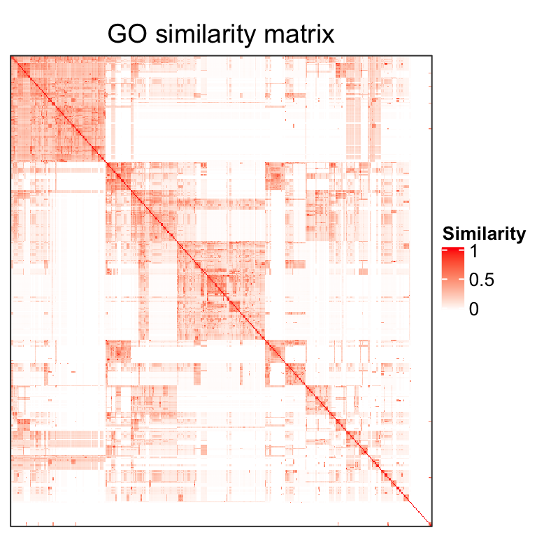
Figure 1. A heatmap of the semantic similarity matrix from 500 random GO terms.

The GO similarity heatmap has a very special pattern that there are blocks located in the diagonal where GO terms in the same block share similar functions. This is due to the structure of the GO relationship which is in a form of the Directed Acyclic Graph (DAG). Terms in a same branch of the graph tend to be more similar where more to the leaves of the graph, the similarity is stronger. In the similarity heatmap, large blocks correspond to the sets of GO terms in large branches or more consentrated to the root of the graph, while small blocks contain GO terms in smaller branches or more to the leaves of the graph.

Classifying GO terms into groups can be thought as a task of clustering the GO simialrity matrix. To solve this problem, there are two types of approaches: 1. the clustering methods that directly apply to a matrix, e.g., k-means clustering, and 2. the methods that treat the similarity matrix as an adjacency matrix and convert the matrix to a weighted graph/network, then graph community/module detection methods are applied to partition the graph.

In the GO graph, there are large branches and small branches, also the branches may have differnet depth in the graph, which causes two major problems for clustering GO terms. First, the sizes of the GO clusters vary a lot, which means, there are very large clusters, and at the same time, there are also many tiny clusters. Large clusters tend to have relatively lower mean similarities across terms while small clusters have relatively higher mean similarity values. Methods such as k-means clustering sometimes cannot preserve the large cluster but further split it into smaller clusters, which might produce redundant information among these smaller clusters. On the other hand, they are not able to separate tiny clusters (see examples in Figure 7). 2. Large GO clusters contain amounts of terms and locate more to the root of the GO graph, which makes it possible that some terms in cluster A also share similarities to terms in cluster B. In the other words, large clusters are less mutually exclusive than small clusters. Some graph community detection methods will merge cluster A and B into a larger cluster. These two problems can be summarized as 1. large clusters are split into small clusters and 2. large clusters are merged into larger cluster. Thus, we need to find an effective method to balance these two scenarios, which is a balance between the generality and specificity of GO clusters.

Here we proposed a new clustering method called “binary cut” to spit GO terms into groups. The idea behind is very simple and staightforward that is to identify “blocks” in the similarity heatmap. As shown in Figure 2, the both two heatmaps are similarity matrices for two subsets of GO terms.

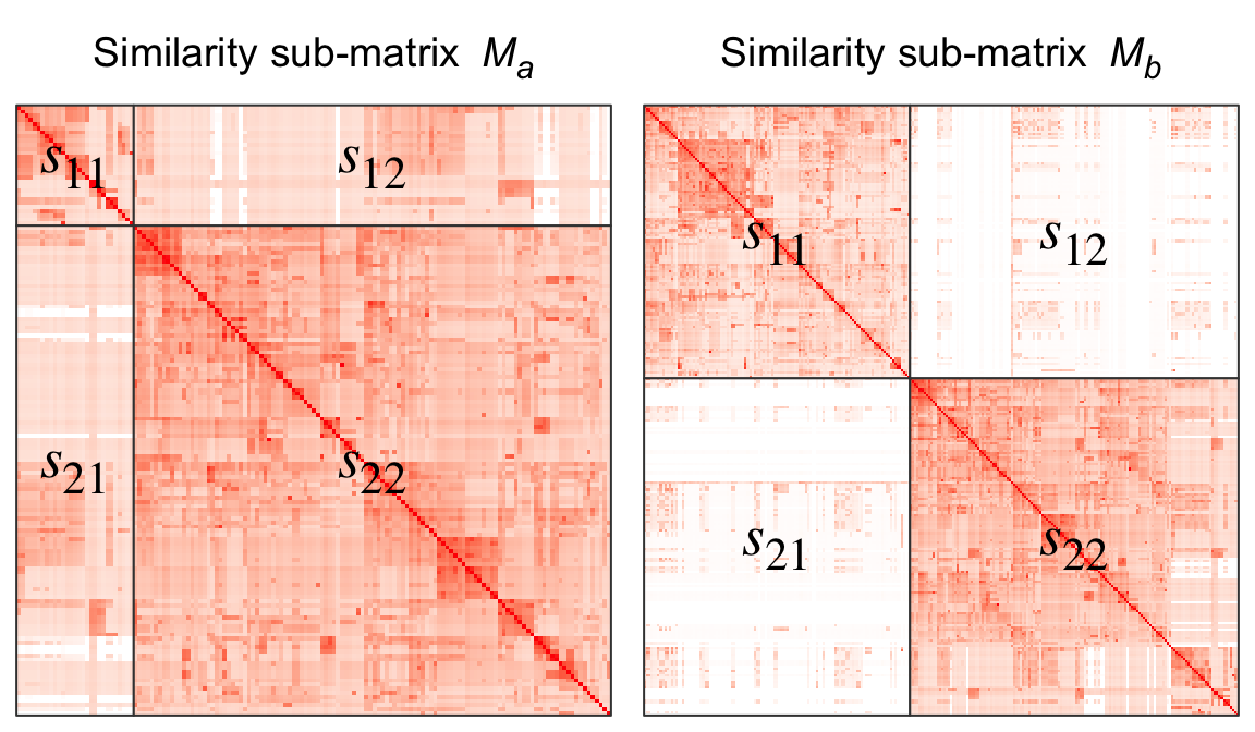
Figure 2. Two similarity matrices that correspond to two subsets of GO terms.

Let’s denote the two matrices as \(M_a\) (the left matrix) and \(M_b\) (the right matrix). Intuitively, terms in \(M_a\) all have high pairwise similarities and thus should be treated as one single cluster and should not be split any more, while terms in \(M_b\) still show two-block pattern and should be further split into two more groups. To measure whether a certain subset of GO terms need to be split, we calculate a score denoted as \(s\) as follows:

For a similarity matrix which corresponds to a subset of GO terms, e.g., \(M_a\) or \(M_b\), k-means clustering with two groups is applied on rows and columns and partitions the matrix into four parts, as illustrated in Figure 2. Denote the score for the four partitions as \(s_{11}\), \(s_{12}\), \(s_{21}\) and \(s_{22}\), where e.g., \(s_{11}\) is the median value of the corresponding sub-matrix, the score \(s\) is calculated as:

\[s = \frac{s_{11} + s_{22}}{s_{11} + s_{12} + s_{21} + s_{22}}\]

Naturally, if \(s\) is close to 0.5 (e.g., the left heatmap), all terms are highly similar and they should not be split any more, while if \(s\) is close to 1, it means the GO terms can still be split into more groups.

The “binary cut” algorithm is composed of two phases:

Phase 1: apply divisive clustering (the top-down approach) and generate a dendrogram.

for a similarity matrix from a set of GO terms, apply k-means clustering with two groups, calculate the score \(s\) and store it on the current node of the dendrogram.
for the two subsets of GO terms partitioned in step 1, apply step 1 to the two sub-matrices respectively.

The clustering in step 1 and 2 are executed recursively untile the number of GO terms in a group reaches 1 which is treated as the leaves of the dendrogram.

Phase 2: cut the dendrogram and generate partitions. Since every node in the dendrogram has a score \(s\) attached, we simply test \(s\) to a cutoff (0.85 as the default). If \(s\) is larger than the cutoff, the two branches from the node is split, or else all the terms under the node are taken as one single cluster.

Nodes with large number of terms tend to have relatively smaller \(s\), thus, it is possible at a certain node, \(s\) does not exceed the cutoff (very close to it), while its child nodes have \(s\) larger than the cutoff. In this case, we don’t want to close the node so early and we still split this node into two subgroups so that its child nodes can be split further more. To overcome this, the rule in phase 2 are modified as: If a node in the dendrogram does not exceed the cutoff, but if at least one of its child nodes exceed the cutoff, the node is still split.

Examples of the step-wise clustering are illustrated in Figure 3 (the first 4 iterations):

Figure 3. Process of binary clustering the similarity matrix. Only the first 4 iterations are shown.

Figure 4 illustrates the complete dendrogram and the partitions in the heatmap. In the dendrogram, for each node, the score \(s\) corresponds to the color of the edge connected to the top of the node. The edges in grey connect the leaves of the dendrogram. The nodes marked with cross lines are the nodes that need to be split under the default cutoff (0.85).

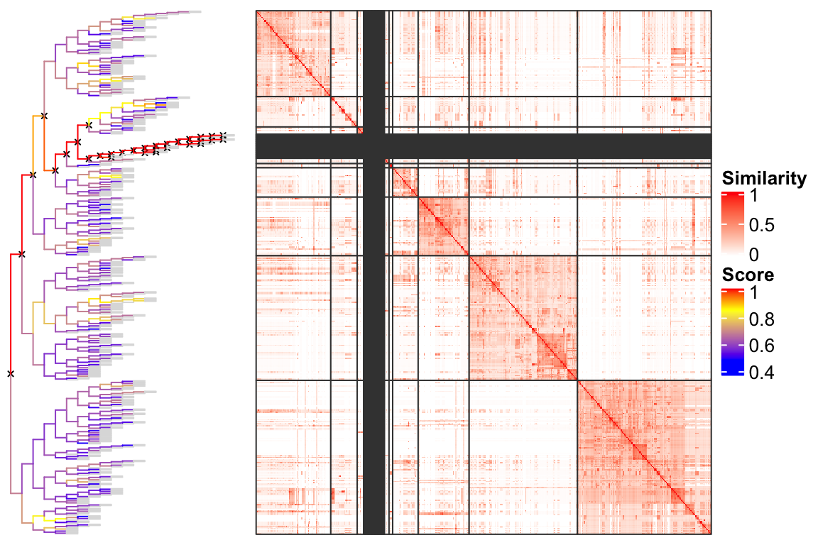
Figure 4. Partition GO terms by splitting the dendrogram.

In Figure 4 we can see there are a lot of tiny clusters that they can actually be put into a separated group. Figure 5 is an improved visualization where clusters with size less than 5 are put into a separated group marked by a green line and moved to the bottom right of the heatmap. This makes the plot looks much more clean.

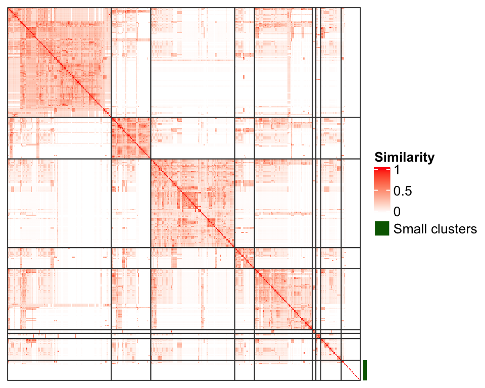
Figure 5. An improved visualization on the clustering of GO terms.

Once the GO terms are clustered into groups, the functions of the terms in each group can be summarized by word clouds of keywords, illustrated in Figure 6.

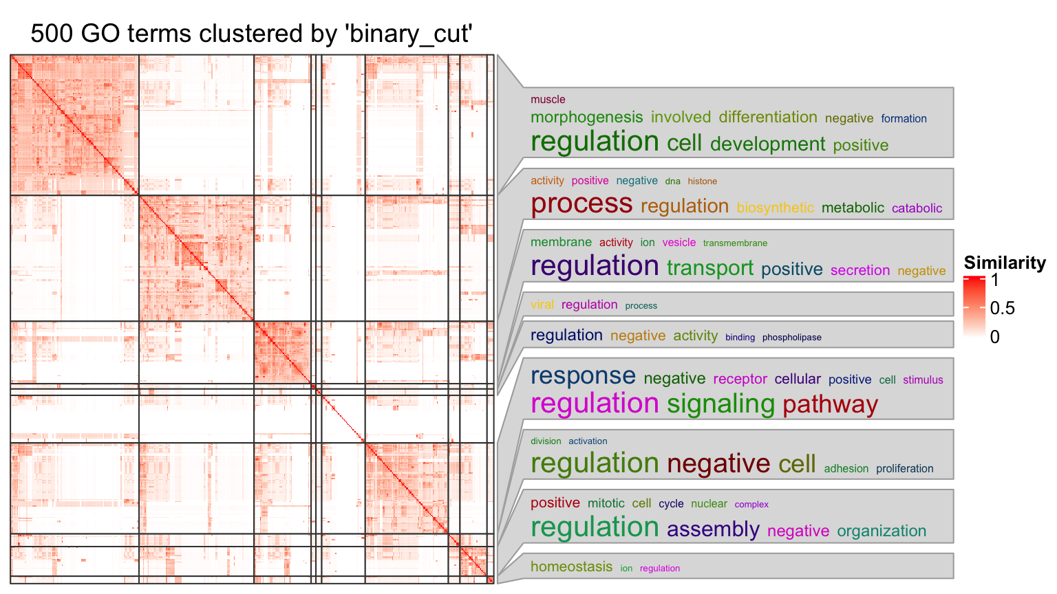
Figure 6. A clustering of GO terms with word clouds as the annotation.

Usage

simplifyGO starts with the GO similarity matrix. Users can use their own similarity matrices or use the GO_similarity() function to calculate one. The GO_similarity() function is simply a wrapper on GOSemSim::termSim. The function accepts a vector of GO IDs. Note the GO should only belong to one same ontology (i.e., BP, CC or MF).

In the following example, we sample 500 random GO IDs from GO Biological Process (BP) ontology.

library(simplifyEnrichment)
set.seed(888)
go_id = random_GO(500)
mat = GO_similarity(go_id)

By default, GO_similarity() uses Rel method in GOSemSim::termSim. Other methods to calculate GO similarities can be set by measure argument, e.g.:

GO_similarity(go_id, measure = "Wang")

With the similarity matrix mat, users can directly apply simplifyGO() function to perform the clustering as well as visualizing the results. The plot is the same as Figure 6, thus here we won’t generate it again in the vignette.

df = simplifyGO(mat)

In simplifyGO(), besides the default clustering method binary_cut, users can also use other clustering methods. The supported methods are:

binary_cut: This is the default clustering method and it uses binary_cut().
kmeans: It uses k-means clustering. The number of clusters are tried with 2:max(2, min(round(nrow(mat)/5), 100)). The best number of k for k-means clustering is identified according to the “elbow” or “knee” method on the distribution of within-cluster sum of squares at each k.
dynamicTreeCut It uses dynamicTreeCut::cutreeDynamic(). The minClusterSize argument is set to 5.
mclust: It uses mclust::Mclust(). The value of G in mclust::Mclust() is set to 1:max(2, min(round(nrow(mat)/5), 100)). Note this method is very time-consuming.
apcluster: It uses apcluster::apcluster(). The s argument is set to apcluster::negDistMat(r = 2).
fast_greedy: It treats the similarity matrix as an adjacency matrix and converts it to a graph where the similarity values are the weight of the edges in the graph. Then the clustering on the similarity matrix is converted to looking for communities in the graph. This method applies igraph::cluster_fast_greedy() to detect communities in the graph.
leading_eigen: It is a graph community detection method. It uses igraph::cluster_leading_eigen().
louvain: It is a graph community detection method. It uses igraph::cluster_louvain().
walktrap: It is a graph community detection method. It uses igraph::cluster_walktrap().

Please note, all other methods are mainly for comparing to the binary_cut method. They are not recommended to use.

On the right side of the heatmap there are the word cloud annotations which summarize the functions with keywords in every GO cluster. Following parameters control the generation and graphic parameters of the word clouds:

draw_word_cloud: Whether to draw the word clouds.
min_term: Minimal number of GO terms in a cluster. All the clusters with size less than min_term are all merged into one single cluster in the heatmap. Default is 5.
order_by_size: Whether to reorder GO clusters by their sizes. The cluster that is merged from small clusters (size < min_term) is always put to the bottom right of the heatmap.
exclude_words: Words that are excluded in the word cloud. E.g., in previous example, the word “regulation” and “process” can be excluded because they have very high frequency in the word clouds but are not very helpful for interpreting the results.
max_words: Maximal number of words visualized in the word cloud, i.e., the top words with the highest frequency.
word_cloud_grob_param: This controls the graphic parameters for the word clouds. The value should be a list and is passed to word_cloud_grob() function. There are following graphic parameters:
- line_space: Space between lines. The value can be a grid::unit object or a numeric scalar which is measured in mm.
- word_space: Space between words. The value can be a grid::unit object or a numeric scalar which is measured in mm.
- max_width: The maximal width of the viewport to put the word cloud. The value can be a grid::unit object or a numeric scalar which is measured in mm. Note this might be larger than the final width of the returned grob object.
- col: Colors for the words. The value should be a self-defined function that takes the number of words and font size as the two arguments. The function should return a color vector. By default it uses random colors.
fontsize_range: The range of the font size. The value should be a numeric vector with length two. The minimal font size is mapped to word frequency value of 1 and the maximal font size is mapped to the maximal word frequency. The font size interlopation is linear.

Note there is no word cloud for the cluster that is merged from small clusters (size < min_term).

The returned variable df is a data frame with GO IDs, GO term names and the cluster labels:

head(df)

##           id                                            term cluster
## 1 GO:0003283                       atrial septum development       1
## 2 GO:0060032                            notochord regression       1
## 3 GO:0031334 positive regulation of protein complex assembly       2
## 4 GO:0097476              spinal cord motor neuron migration       1
## 5 GO:1901222           regulation of NIK/NF-kappaB signaling       3
## 6 GO:0018216                   peptidyl-arginine methylation       4

The size of GO clusters can be retrieved by:

sort(table(df$cluster))

## 
##   6   7  11  12  15  16  18  20  21  23  25  26  28  29  30  31  32  33  34  35  36  37  38  39  40 
##   1   1   1   1   1   1   1   1   1   1   1   1   1   1   1   1   1   1   1   1   1   1   1   1   1 
##  41  42  17  22  24   8  10  13  19  27  14   9   2   5   3   4   1 
##   1   1   2   2   2   4   4   4   5   6   7  12  28  59  86 119 133

Or split the data frame by the cluster labels:

split(df, df$cluster)

plot argument can be set to FALSE in simplifyGO(), so that no plot is generated and only the data frame is returned.

If the aim is only to cluster GO terms, binary_cut() function can be directly applied:

binary_cut(mat)

##   [1]  1  1  2  1  3  4  5  4  1  4  6  5  1  4  5  4  1  4  1  4  1  1  7  8  1  4  4  3  4  3  3
##  [32]  4  3  1  4  1  4  4  3  1  4  3  4  1  9  4  5  1 10  2  1  4  3  3  3  1  4  3  3  4  3  5
##  [63]  1  4  4  4  1  4  3  1  3 11  1  5  1 12  2 10  4  1  3 13 14  1  1  3  1  5  3 15  1  1  3
##  [94]  4  4  4  3  4 10  1  1 10 10  5  2  3  1  2  3  3  1  3 16  1  3  3  1  4  2  4  3 17  1  4
## [125]  3  2  2  4  3 10  4  4 18  5  2  2  1  1  4  1  4  5  2  1  1 19  1  1  4  1  2 20  3  1  1
## [156]  1  1  4  1  1  1  4 10  1  2  1  5  3  1  5  3  4  1  3  3  3  4  1  1 12  5  3  3 13  3  1
## [187]  5  8  3  1  3 21  4  1  4  2  1  1  1 12  1  1  4  3  3  2  1  3  4  4  1  3  4  5  5  1 22
## [218] 13  3 17  2  4  2  4  2  2  4  2  1  1  4  2  1  5  4 10  4  3  5  3  1 23  3  1  4  1  1  3
## [249]  5  3 10  1  1  1  4  1  3  3  4  3  1 24  1  1 25  8  9  4  3  5  3  1  1 23  4 26  5  3  5
## [280]  1  1  4  4  5  1  3  3  2  3 17  4  4  4 20  8  4  3  3  4 12  4  1  1  9  2  3  1  1  2  1
## [311]  1  2  4  4  1  1  4  4  4  1  3  3 27  5  3  3  3  2  1  1  1  3  1  4  2  4  4  3  3  3  1
## [342]  3  1  4  1  4  1 13  3  1  5 13  1  1  3  1  1  4  1  1  2  4  1  4  4  4  1  1  3  1  4 13
## [373]  4  1  4  4  3  3  4  1  2  5  4  5  4  4  4 28  4  4  3  4  1  3  2  3  2 29  4  3  1  2  1
## [404]  1  2 10  4  3  1  2  1  3  1  5  1  4  3  5 23  1  3 23  4  3  3 30  1  4  3  1  4 15 23 17
## [435]  4  4  9  1  1  3  5  1  4  1  5  4  1  1  1 31  1  3  3  1 13  1  1  4  4  4  5  3 32  2  4
## [466]  4  5 33  3  1  4  1  3  1  1  1  4  1  1  4  4  1  1  4  4  4  8 34 23  3  4  4  4 35 36  3
## [497]  5  3 37  5

Benchmark

We compare the following clustering methods to binary cut: kmeans, dynamicTreeCut, mclust, apcluster, fast_greedy, leading_eigen, louvain and walktrap. The actual R functions used to perform corresponding analysis can be found in text in previous sections in this vignette.

On random datasets

500 random GO terms are generated from Biology Process ontology. One example of the clusterings from different methods is illustrated in Figure 7. Basically we can see kmeans, dynamicTreeCut, mclust and apcluster generate too many small clusters. fast_greedy, leading_eigen, louvain and walktrap can identify both small and large clusters, however, some large clusters should still need to be split further more.

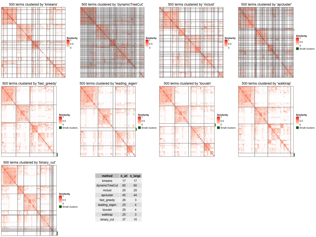
Figure 7. Compare clustering from different methods. Tiny clusters (size < 5) are merged into a separated cluster marked by a green line.

We use the following metrics to benchmark the clustering methods:

Different score: This is the difference between the similarity values for the terms that belong to the same clusters and different clusters. For a similarity matrix \(M\), for term \(i\) and term \(j\) where \(i \ne j\), the similarity value \(x_{i,j}\) is saved to the vector \(\mathbf{x_1}\) only when term \(i\) and \(j\) are in a same cluster. \(x_{i,j}\) is saved to the vector \(\mathbf{x_2}\) when term \(i\) and \(j\) are not in the same cluster. The difference score measures the distribution difference between \(\mathbf{x_1}\) and \(\mathbf{x_2}\), calculated as the Kolmogorov-Smirnov statistic between the two distributions.
Number of clusters: For each clustering, there are two numbers: the number of total clusters and the number of clusters with size >= 5 (only the big clusters).
Block mean: The mean similarity values of the blocks in the similarity heatmap. Similar denotation as difference score, for term \(i\) and \(j\) where \(i\) can be the same as \(j\) (values on the diagonal are also used), the similarity value \(x_{i,j}\) is saved to the vector \(\mathbf{x_3}\) only when term \(i\) and \(j\) are in a same cluster. The block mean is the mean value over \(\mathbf{x_3}\).

The random GO terms were generated 100 times and the metrics are compared in Figure 8.

In the left plot in Figure 8, in the top panel, we can see binary cut has the highest difference score, which means, in the clustering by binary cut, the terms in the same clusters shows the most distinct distribution to the rest of values in the similarity matrix. In the middle panel, dynamicTreeCut and apcluster generates huge number of clusters, as we already see in Figure 7. They are just too stringent to cluster GO terms that the clusters should have very high redundant information. As a comparison, community-based methods and binary cut generate moderate number of clusters, especially, the number of “big cluster” (those with size >= 5) drops dramatically compare to the total clusters, indicating these methods are able to identify tiny clusters that have very low similarity to any other terms. In the bottom panel, Binary cut generates clusters with moderate “block mean”. As a comparison, kmeans, dynamicTreeCut, mclust and apcluster generate very high block mean, which associates to the huge amount of small clusters by these methods, and community detection methods generate very low block mean, which is mainly because terms in some of the large clusters have almost no similarities and these large clusters should be still split into smaller ones. This comparison indicates binary cut keeps both generality and flexibility of GO clusters.

Next we look at the similarity between clustering methods. For the clusterings from two methods, first the cluster labels are adjusted. Denote \(\mathbf{s_1}\) as the label vector for method 1, \(\mathbf{s_2}\) as the label vector for method 2, and \(\mathbf{s_1}\) as the reference labels, we apply clue::solve_LSAP() function generate a mapping function \(m()\) between the two sets of labels to maximize \(\sum^n_i I(s_{1i}, m(s_{2i}))\) where \(n\) is the length of \(\mathbf{s_1}\) or \(\mathbf{s_2}\). Denote the adjusted labels for the second method as \(s'_{2i} = m(s_{2i})\), the concordance between the two clusterings are calculated as:

\[ \frac{1}{n}\sum_i^n I(s_{1i}, s'_{2i}) \]

where \(I(x, y)\) is an indicator function with value 1 if \(x = y\) and 0 if \(x \ne y\). A concordance of 1 means the two clusterings are identical.

Right plot in Figure 8 illustrates the heatmap for the mean concordance of the clusterings from 500 runs on the random GO datasets. We see binary cut is more similar as the community detection methods.

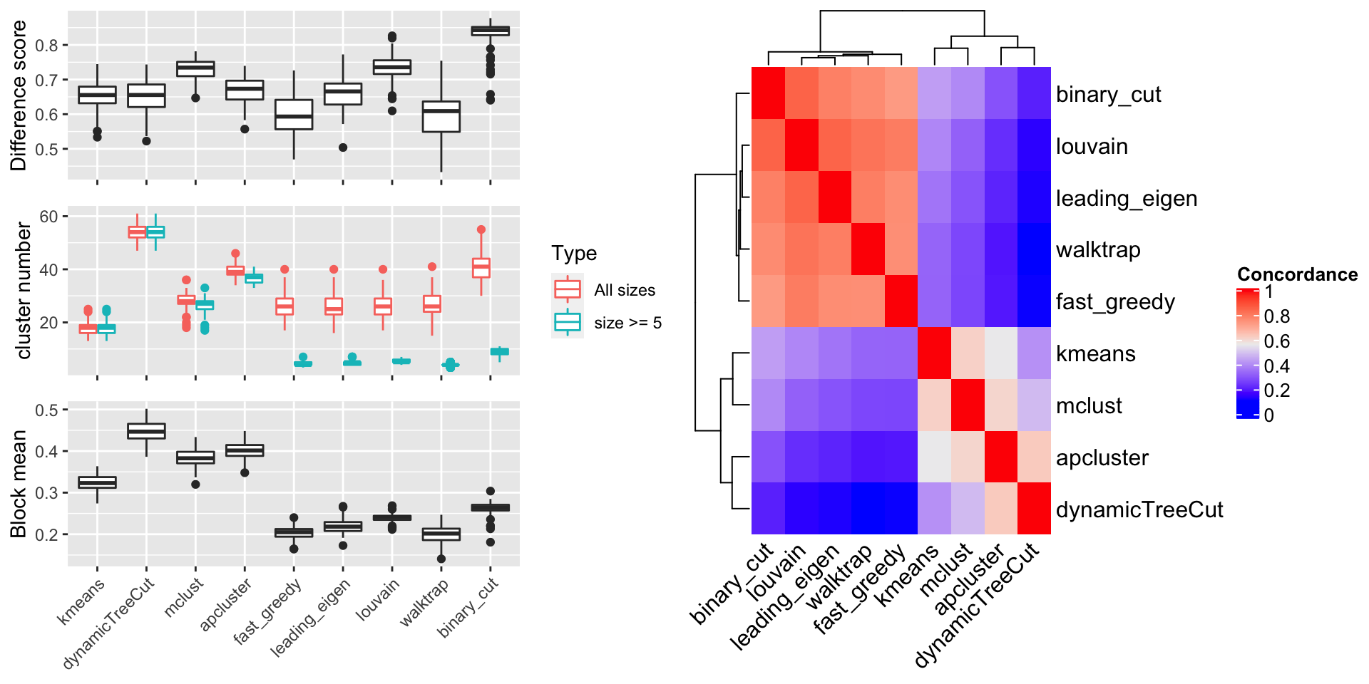
Figure 8. Compare metrics for different clustering methods, on randomly generated datasets.

The heatmaps for the 100 runs of clustering random GO terms can be found at https://jokergoo.github.io/simplifyGO_figures/random_BP.html.

On real datasets

We downloaded the datasets from EBI Expression Atlas. We applied clusterProfiler to the significantly expressed genes (FDR < 0.05) only with the GO Biological Process ontology. We only took the datasets with number of significant genes in [500, 3000] and number of significant GO terms in [100, 1000]. Finally there are 475 GO lists.

Figure 9 illustrates the results for the comparison. The conclusion is basically the same as the random GO datasets.

The heatmaps for all datasets can be found at https://jokergoo.github.io/simplifyGO_figures/EBI_Expression_Atlas.html.

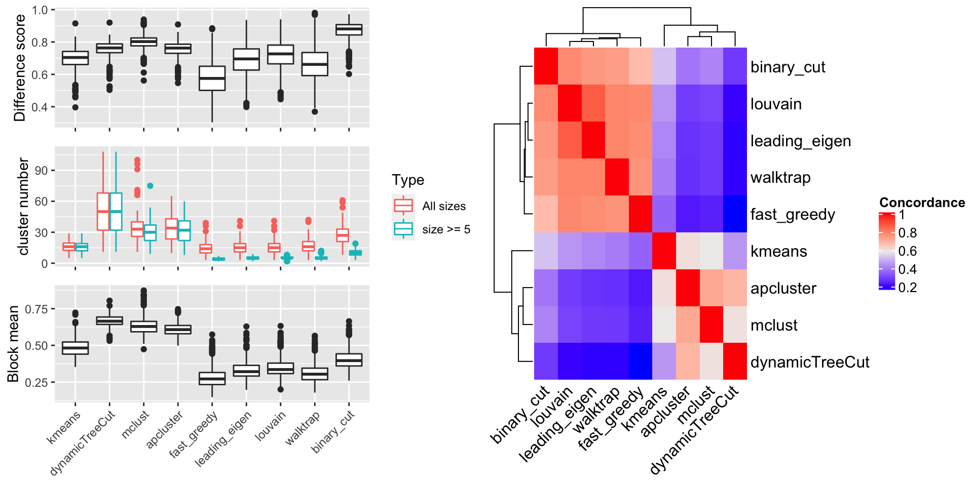
Figure 9. Compare metrics for different clustering methods, on real-world datasets.

Utility functions for comparing clustering methods

In the simplifyEnrichment package, there are also functions that compare clustering results from different methods. Here we still use previously generated variable mat which is the similarity matrix from the 500 random GO terms. Simply running compare_methods() function performs all supported methods (in all_clustering_methods()) excluding mclust, because mclust usually takes very long time to run. The function generates a figure with three panels:

A heatmap of the similarity matrix with different clusterings as row annotations.
A heatmap of the pair-wise concordance of the clustering from every two methods.
Barplots of the difference scores for each method, the number of clusters (total clusters and the clusters with size >= 5) and the mean similarity of the terms that are in the same clusters (block mean). The methods to calculate these metrics are introduced in the previous section.

compare_methods(mat)

## cluster 500 terms by kmeans... 17 clusters.
## cluster 500 terms by dynamicTreeCut... 60 clusters.
## cluster 500 terms by apcluster... 45 clusters.
## cluster 500 terms by fast_greedy... 26 clusters.
## cluster 500 terms by leading_eigen... 25 clusters.
## cluster 500 terms by louvain... 25 clusters.
## cluster 500 terms by walktrap... 25 clusters.
## cluster 500 terms by binary_cut... 38 clusters.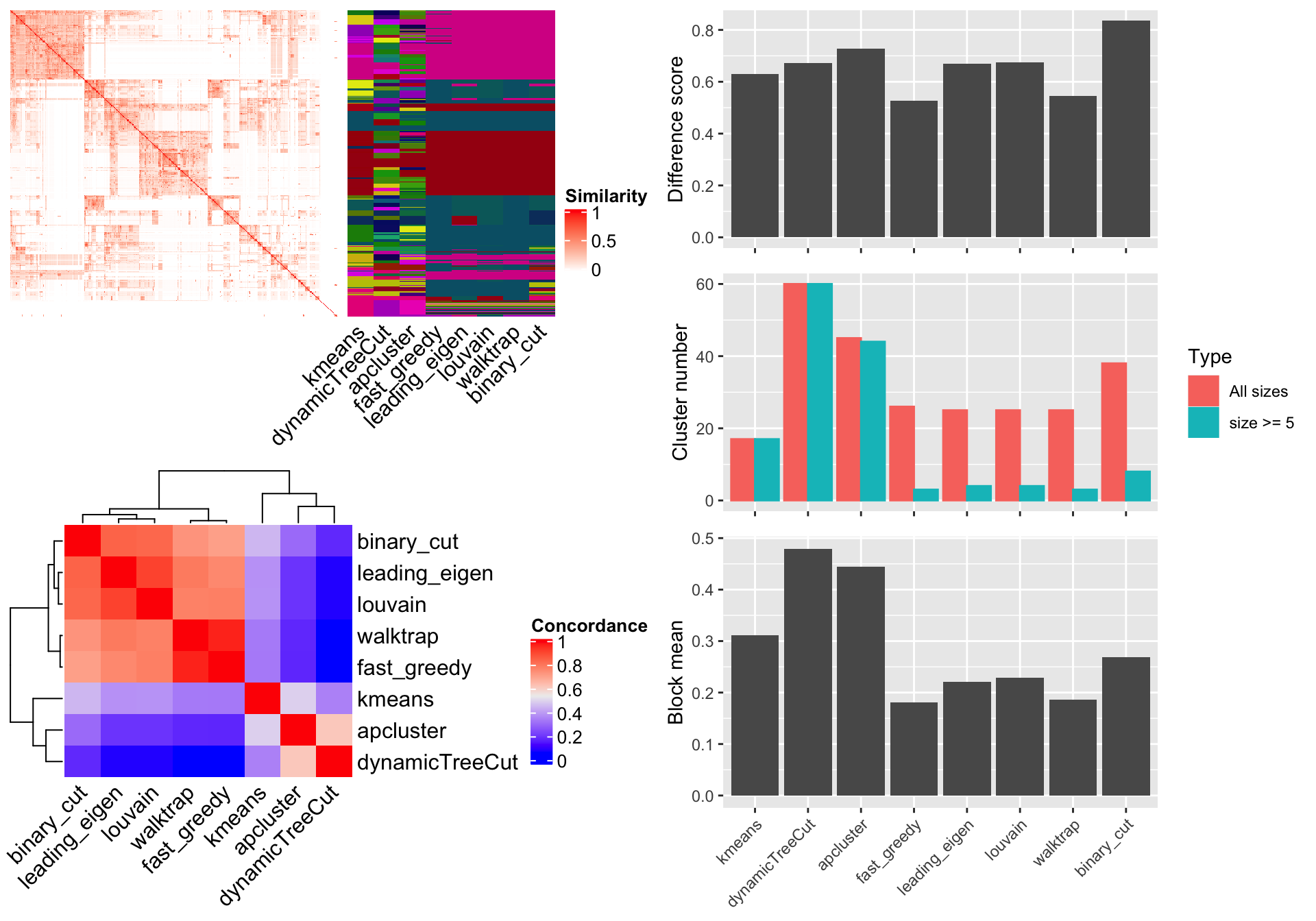

Figure 10. Compare different clustering methods.

If plot_type argument is set to heatmap. There are heatmaps for the similarity matrix under different clusterings methods. The last panel is a table with the number of clusters. nrow argument controls the number of rows in the layout. An example can be found in Figure 7.

# The following code may take long time to run (several minutes)
compare_methods(mat, plot_type = "heatmap")
compare_methods(mat, plot_type = "heatmap", nrow = 3)

Please note, the clustering methods might have randomness, which means, different runs of compare_methods() may generate different clusterings (slightly different). Thus, if users want to compare the plots between compare_methods(mat) and compare_methods(mat, plot_type = "heatmap"), they should set the same random seed before executing the function.

set.seed(123)
compare_methods(mat)
set.seed(123)
compare_methods(mat, plot_type = "heatmap")

compare_methods() is simply a wrapper on compare_methods_make_clusters() and compare_methods_make_plot() functions where the former function performs clustering with different methods and the latter visualizes the results. To compare different plots, users can also use the following code without specifying the random seed.

clt = compare_methods_make_clusters(mat) # just a list of cluster labels
compare_methods_make_plot(mat, clt)
compare_methods_make_plot(mat, clt, plot_type = "heatmap")

Register new clustering methods

New clustering methods can be added by register_clustering_methods(), removed by remove_clustering_methods() and reset to the default methods by reset_clustering_methods(). All the supported methods can be retrieved by all_clustering_methods(). compare_methods() runs all the clustering methods in all_clustering_methods().

The new clustering methods should be as user-defined functions and sent to register_clustering_methods() as named arguments, e.g.:

register_clustering_methods(
    method1 = function(mat, ...) ...,
    method2 = function(mat, ...) ...,
    ...
)

The functions should accept at least one argument which is the input matrix (mat in above example). The second optional argument should always be ... so that parameters for the clustering function can be passed by control argument from cluster_terms() or simplifyGO(). If users forget to add ..., it is added internally.

Please note, the user-defined function should automatically identify the optimized number of clusters. The function should return a vector of cluster labels. Internally it is converted to numeric labels.

Session Info

sessionInfo()

## R version 4.0.0 (2020-04-24)
## Platform: x86_64-apple-darwin17.0 (64-bit)
## Running under: macOS Catalina 10.15.4
## 
## Matrix products: default
## BLAS:   /Library/Frameworks/R.framework/Versions/4.0/Resources/lib/libRblas.dylib
## LAPACK: /Library/Frameworks/R.framework/Versions/4.0/Resources/lib/libRlapack.dylib
## 
## locale:
## [1] en_GB.UTF-8/en_GB.UTF-8/en_GB.UTF-8/C/en_GB.UTF-8/en_GB.UTF-8
## 
## attached base packages:
##  [1] parallel  stats4    grid      stats     graphics  grDevices utils     datasets  methods  
## [10] base     
## 
## other attached packages:
##  [1] ggplot2_3.3.0             cowplot_1.0.0             org.Hs.eg.db_3.10.0      
##  [4] AnnotationDbi_1.50.0      IRanges_2.22.1            S4Vectors_0.26.0         
##  [7] Biobase_2.48.0            BiocGenerics_0.34.0       ComplexHeatmap_2.5.2     
## [10] circlize_0.4.9            simplifyEnrichment_0.99.0 knitr_1.28               
## 
## loaded via a namespace (and not attached):
##  [1] dynamicTreeCut_1.63-1 bit64_0.9-7           assertthat_0.2.1      highr_0.8            
##  [5] blob_1.2.1            yaml_2.2.1            slam_0.1-47           lattice_0.20-41      
##  [9] pillar_1.4.3          RSQLite_2.2.0         backports_1.1.6       glue_1.4.0           
## [13] digest_0.6.25         RColorBrewer_1.1-2    gridtext_0.1.1        colorspace_1.4-1     
## [17] htmltools_0.4.0       Matrix_1.2-18         tm_0.7-7              pkgconfig_2.0.3      
## [21] GetoptLong_0.1.8      purrr_0.3.4           GO.db_3.10.0          scales_1.1.0         
## [25] jpeg_0.1-8.1          tibble_3.0.1          farver_2.0.3          ellipsis_0.3.0       
## [29] withr_2.2.0           NLP_0.2-0             magrittr_1.5          crayon_1.3.4         
## [33] memoise_1.1.0         evaluate_0.14         apcluster_1.4.8       fs_1.4.1             
## [37] MASS_7.3-51.6         xml2_1.3.2            tools_4.0.0           GlobalOptions_0.1.1  
## [41] lifecycle_0.2.0       stringr_1.4.0         munsell_0.5.0         cluster_2.1.0        
## [45] compiler_4.0.0        pkgdown_1.5.1         gridGraphics_0.5-0    rlang_0.4.5          
## [49] rjson_0.2.20          igraph_1.2.5          labeling_0.3          rmarkdown_2.1        
## [53] gtable_0.3.0          DBI_1.1.0             markdown_1.1          R6_2.4.1             
## [57] dplyr_0.8.5           bit_1.1-15.2          clue_0.3-57           rprojroot_1.3-2      
## [61] shape_1.4.4           desc_1.2.0            GOSemSim_2.14.0       stringi_1.4.6        
## [65] Rcpp_1.0.4.6          vctrs_0.2.4           png_0.1-7             tidyselect_1.0.0     
## [69] xfun_0.13

Zuguang Gu (z.gu@dkfz.de)

2020-05-10