Draw horizon chart along the spiral

spiral_horizon(x, y, y_max = max(abs(y)), n_slices = 4, slice_size,
    pos_fill = "#D73027", neg_fill = "#313695",
    use_bars = FALSE, bar_width = min(diff(x)),
    negative_from_top = FALSE, track_index = current_track_index())

Arguments

x: X-locations of the data points.
y: Y-locations of the data points.
y_max: Maximal absolute value on y-axis.
n_slices: Number of slices.
slice_size: Size of the slices. The final number of sizes is ceiling(max(abs(y))/slice_size).
pos_fill: Colors for positive values.
neg_fill: Colors for negative values.
use_bars: Whether to use bars?
bar_width: Width of bars.
negative_from_top: Should negative distribution be drawn from the top?
track_index: Index of the track.

Details

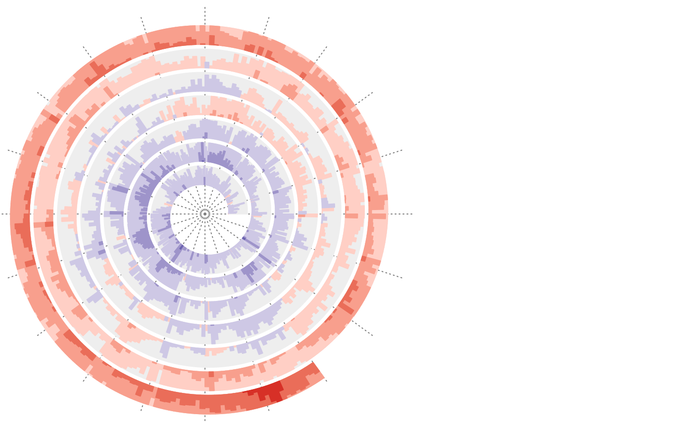
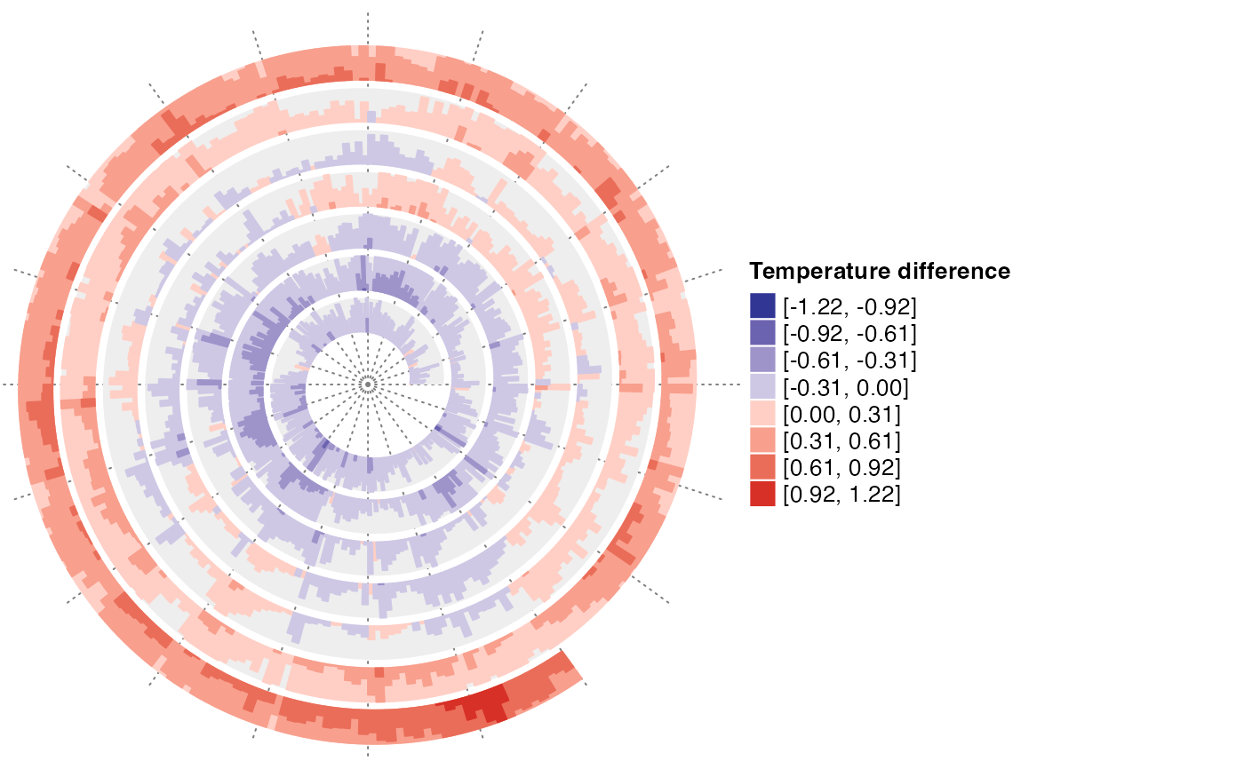
Since the track height is very small in the spiral, horizon chart visualization is a efficient way to visualize distribution-like graphics.

Value

A list of the following objects:

a color mapping function for colors.
a vector of intervals that split the data.

Examples

# \donttest{
df = readRDS(system.file("extdata", "global_temperature.rds", package = "spiralize"))
df = df[df$Source == "GCAG", ]
spiral_initialize_by_time(xlim = range(df$Date), unit_on_axis = "months", period = "year",
    period_per_loop = 20, polar_lines_by = 360/20, 
    vp_param = list(x = unit(0, "npc"), just = "left"))
spiral_track()
spiral_horizon(df$Date, df$Mean, use_bar = TRUE)

# }