Simplify Functional Enrichment Results
Zuguang Gu (z.gu@dkfz.de)
2024-09-13
Source:vignettes/simplifyEnrichment_intro.Rmd
simplifyEnrichment_intro.RmdThe simplifyEnrichment package clusters functional terms into groups by clustering the similarity matrix of the terms with a new proposed method “binary cut” which recursively applies partition around medoids (PAM) with two groups on the similarity matrix and in each iteration step, a score is assigned to decide whether the group of gene sets that corresponds to the current sub-matrix should be split or not. For more details of the method, please refer to the simplifyEnrichment paper.
Simplify GO enrichment results
The major use case for simplifyEnrichment is for simplying the GO enrichment results by clustering the corresponding semantic similarity matrix of the significant GO terms. To demonstrate the usage, we first generate a list of random GO IDs from the Biological Process (BP) ontology category:
library(simplifyEnrichment)
set.seed(888)
go_id = random_GO(500)
simplifyEnrichment starts with the GO similarity matrix. Users can use their own similarity matrices or use the GO_similarity() function to calculate the semantic similarity matrix. The GO_similarity() function is simply a wrapper on GOSemSim::termSim(). The function accepts a vector of GO IDs. Note the GO terms should only belong to one same ontology (i.e., BP, CC or MF).
mat = GO_similarity(go_id)By default, GO_similarity() uses Rel method in GOSemSim::termSim(). Other methods to calculate GO similarities can be set by measure argument, e.g.:
GO_similarity(go_id, measure = "Wang")With the similarity matrix mat, users can directly apply simplifyGO() function to perform the clustering as well as visualizing the results.
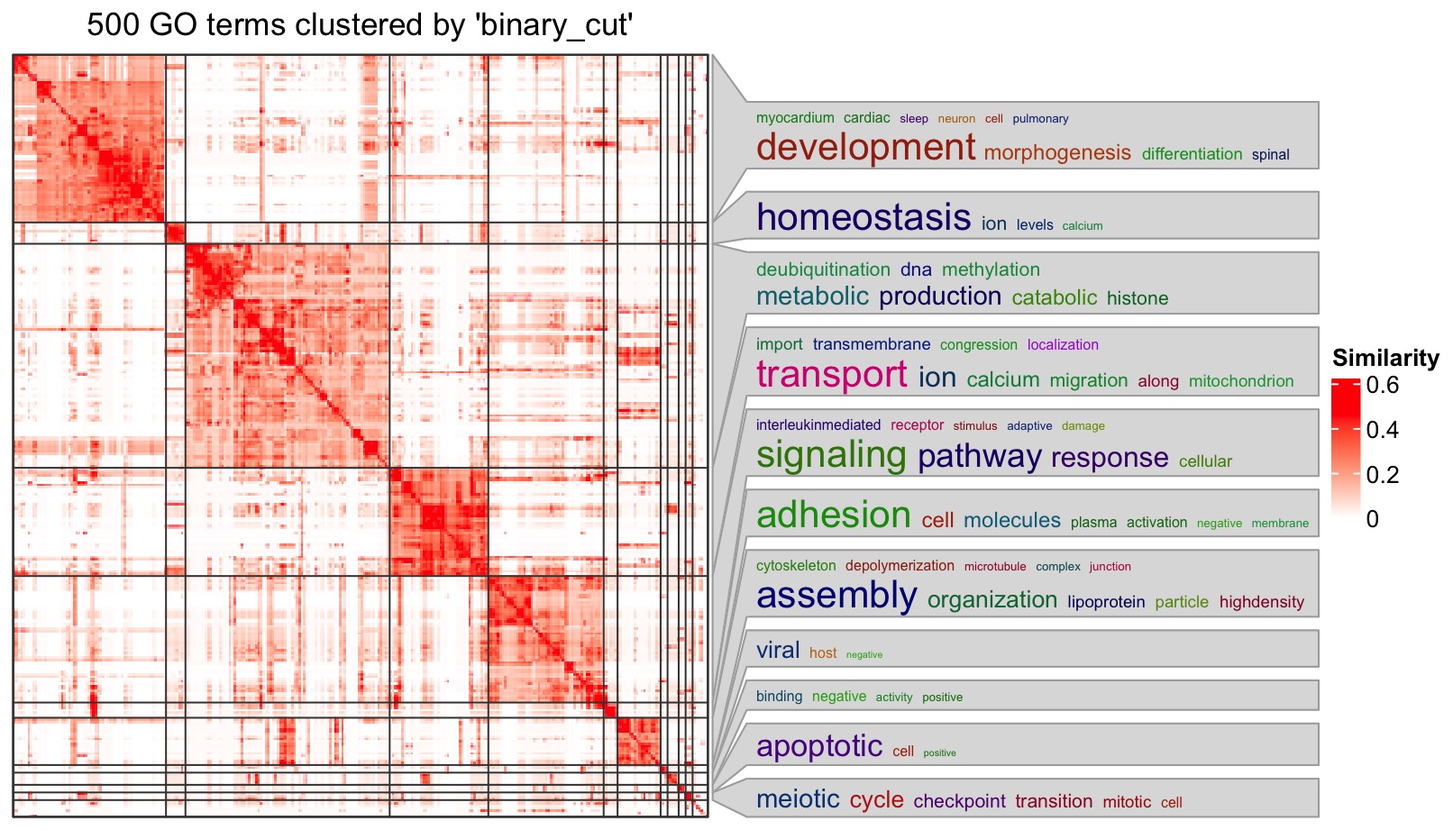
df = simplifyGO(mat)
On the right side of the heatmap there are the word cloud annotations which summarize the functions with keywords in every GO cluster. Additionally, enrichment is done on keywords compared to GO background vocabulary and the significance corresponds to the font size of the keywords.
Note there is no word cloud for the cluster that is merged from small clusters (size < 5).
The returned variable df is a data frame with GO IDs and the cluster labels:
head(df)## id cluster
## 1 GO:0086066 1
## 2 GO:0090461 2
## 3 GO:0032912 3
## 4 GO:0090220 4
## 5 GO:0032495 5
## 6 GO:0070585 4The size of GO clusters can be retrieved by:
##
##  15  16  17  18  19   8   9  14  10  12  13  11   6   2   7   4   5   1   3
##   1   1   1   1   1   2   2   2   5   5   5   8  10  14  31  71  83 110 147
Or split the data frame by the cluster labels:
split(df, df$cluster)plot argument can be set to FALSE in simplifyGO(), so that no plot is generated and only the data frame is returned.
If the aim is only to cluster GO terms, binary_cut() or cluster_terms() functions can be directly applied:
binary_cut(mat)## [1] 1 2 3 4 5 4 4 4 1 3 3 5 1 5 1 4 1 4 5 4 5 1 4 3 6
## [26] 3 7 4 3 1 1 3 8 7 3 3 5 1 4 4 5 2 4 9 5 1 1 7 3 7
## [51] 5 3 10 7 1 7 3 10 3 3 7 1 5 5 3 1 1 1 1 3 1 4 11 3 1
## [76] 3 4 7 3 3 1 5 4 6 3 3 1 5 4 5 7 3 3 4 5 3 1 1 4 6
## [101] 4 3 4 4 1 4 3 5 3 7 3 1 3 3 3 1 1 1 9 4 4 8 3 1 1
## [126] 1 1 5 4 1 4 1 3 5 5 5 1 5 3 5 5 5 1 3 5 5 12 1 2 4
## [151] 8 3 7 1 3 5 8 1 4 5 1 5 1 1 5 3 3 4 1 1 3 3 3 1 4
## [176] 4 1 3 4 3 3 13 5 4 4 3 1 3 5 3 5 3 3 3 1 1 1 5 4 3
## [201] 2 5 4 4 2 3 1 1 3 3 1 2 3 3 3 4 5 3 4 3 4 6 6 4 7
## [226] 4 5 5 1 1 3 1 10 8 7 7 5 5 3 3 7 3 1 4 1 1 5 6 3 5
## [251] 5 1 14 1 3 11 4 1 5 12 3 1 7 3 1 5 1 3 5 5 3 6 1 5 3
## [276] 11 1 2 3 4 5 12 1 1 10 3 5 3 3 3 7 4 5 3 3 4 1 1 4 7
## [301] 3 2 4 5 3 3 5 3 1 3 2 5 2 3 3 1 1 5 5 4 11 1 1 5 3
## [326] 3 1 4 5 1 1 1 1 7 3 2 3 2 5 3 5 1 12 3 3 4 3 1 4 6
## [351] 4 7 1 3 1 4 7 3 5 3 1 2 11 4 3 3 1 1 1 5 7 7 1 1 3
## [376] 5 3 7 3 10 1 3 1 7 3 1 3 11 3 15 4 6 3 1 3 7 6 1 5 4
## [401] 5 3 1 3 3 5 3 3 7 4 5 1 7 5 7 3 1 8 3 3 10 1 1 4 3
## [426] 1 3 12 1 3 3 1 1 5 3 3 1 1 1 1 16 5 1 3 7 3 1 5 1 5
## [451] 7 3 4 5 4 4 1 1 3 5 7 11 4 4 5 3 4 4 1 1 3 5 8 5 3
## [476] 3 3 3 5 17 3 3 3 4 1 11 5 1 3 3 1 5 3 1 3 18 7 5 3 1or
cluster_terms(mat, method = "binary_cut")binary_cut() and cluster_terms() basically generate the same clusterings, but the labels of clusters might differ.
Comparing clustering methods
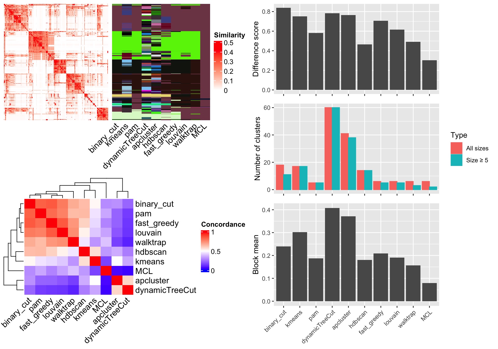
In the simplifyEnrichment package, there are also functions that compare clustering results from different methods. Here we still use previously generated variable mat which is the similarity matrix from the 500 random GO terms. Simply running compare_clustering_methods() function performs all supported methods (in all_clustering_methods()) excluding mclust, because mclust usually takes very long time to run. The function generates a figure with three panels:
- A heatmap of the similarity matrix with different clusterings as row annotations.
- A heatmap of the pair-wise concordance of the clustering from every two methods.
- Barplots of the difference scores for each method, the number of clusters (total clusters and the clusters with size >= 5) and the mean similarity of the terms that are in the same clusters (block mean).
In the barplots, the three metrics are defined as follows:
- Different score: This is the difference between the similarity values for the terms that belong to the same clusters and different clusters. For a similarity matrix \(M\), for term \(i\) and term \(j\) where \(i \ne j\), the similarity value \(x_{i,j}\) is saved to the vector \(\mathbf{x_1}\) only when term \(i\) and \(j\) are in a same cluster. \(x_{i,j}\) is saved to the vector \(\mathbf{x_2}\) when term \(i\) and \(j\) are not in the same cluster. The difference score measures the distribution difference between \(\mathbf{x_1}\) and \(\mathbf{x_2}\), calculated as the Kolmogorov-Smirnov statistic between the two distributions.
- Number of clusters: For each clustering, there are two numbers: the number of total clusters and the number of clusters with size >= 5 (only the big clusters).
- Block mean: Mean similarity values of the diagonal blocks in the similarity heatmap. Using the same convention as for the difference score, the block mean is the mean value of \(\mathbf{x_1}\).

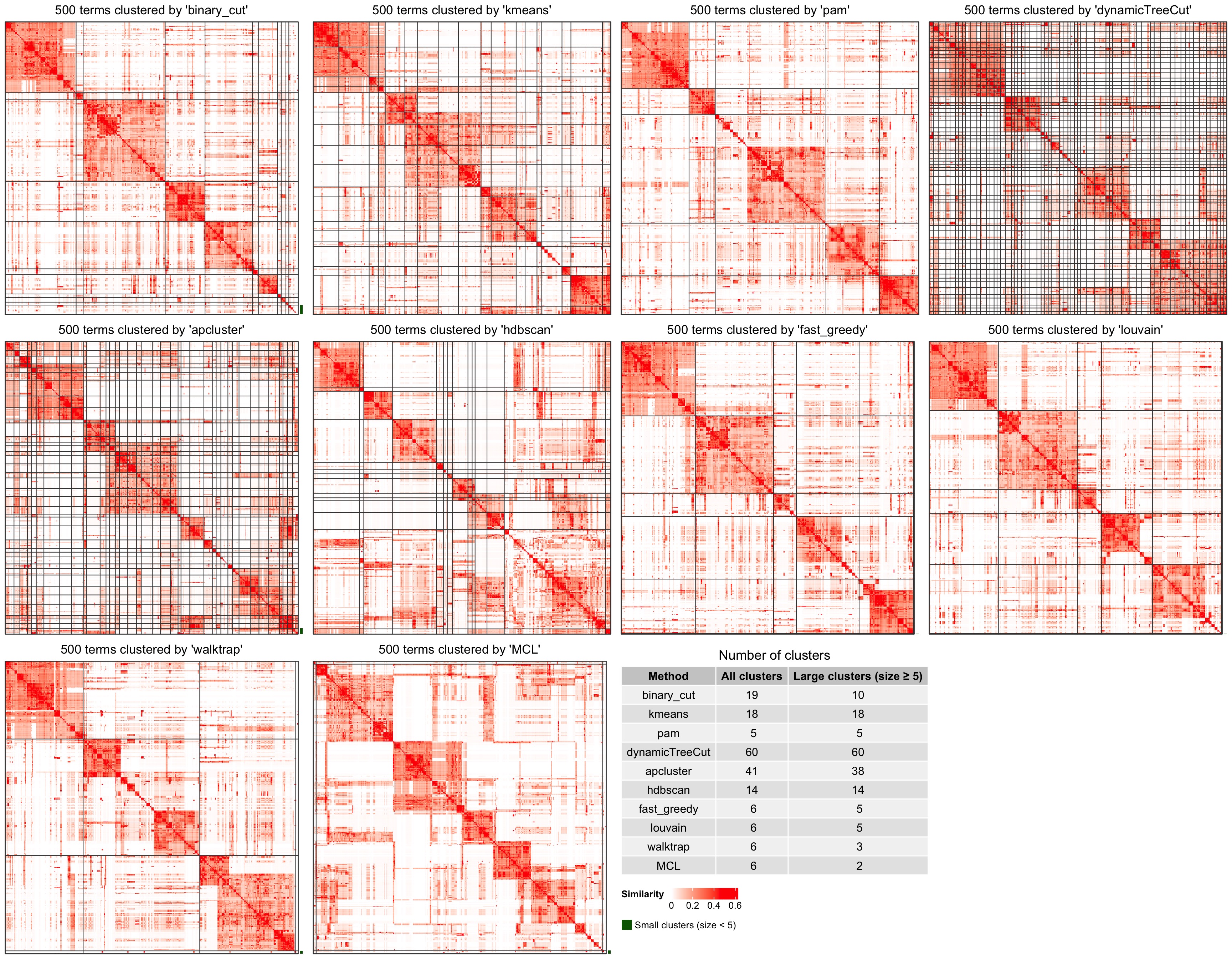
If plot_type argument is set to heatmap. There are heatmaps for the similarity matrix under different clusterings methods. The last panel is a table with the number of clusters.
compare_clustering_methods(mat, plot_type = "heatmap")
Please note, the clustering methods might have randomness, which means, different runs of compare_clustering_methods() may generate different clusterings (slightly different). Thus, if users want to compare the plots between compare_clustering_methods(mat) and compare_clustering_methods(mat, plot_type = "heatmap"), they should set the same random seed before executing the function.
set.seed(123)
compare_clustering_methods(mat)
set.seed(123)
compare_clustering_methods(mat, plot_type = "heatmap")
compare_clustering_methods() is simply a wrapper on cmp_make_clusters() and cmp_make_plot() functions where the former function performs clustering with different methods and the latter visualizes the results. To compare different plots, users can also use the following code without specifying the random seed.
clt = cmp_make_clusters(mat) # just a list of cluster labels
cmp_make_plot(mat, clt)
cmp_make_plot(mat, clt, plot_type = "heatmap")
Register new clustering methods
New clustering methods can be added by register_clustering_methods(), removed by remove_clustering_methods() and reset to the default methods by reset_clustering_methods(). All the supported methods can be retrieved by all_clustering_methods(). compare_clustering_methods() runs all the clustering methods in all_clustering_methods().
The new clustering methods should be as user-defined functions and sent to register_clustering_methods() as named arguments, e.g.:
register_clustering_methods(
    method1 = function(mat, ...) ...,
    method2 = function(mat, ...) ...,
    ...
)
The functions should accept at least one argument which is the input matrix (mat in above example). The second optional argument should always be ... so that parameters for the clustering function can be passed by control argument from cluster_terms() or simplifyGO(). If users forget to add ..., it is added internally.
Please note, the user-defined function should automatically identify the optimized number of clusters. The function should return a vector of cluster labels. Internally it is converted to numeric labels.
Apply to multiple lists of GO IDs
It is always very common that users have multiple lists of GO enrichment results (e.g. from multiple groups of genes) and they want to compare the significant terms between different lists, e.g. to see which biological functions are more specific in a certain list. There is a function simplifyGOFromMultipleLists() in the package which helps this type of analysis.
The input data for simplifyGOFromMultipleLists() (with the argument lt) can have three types of formats:
- A list of numeric vectors of adjusted p-values where each vector has the GO IDs as names.
- A data frame. The column of the GO IDs can be specified with
go_id_columnargument and the column of the adjusted p-values can be specified withpadj_columnargument. If the two columns are not specified, they are automatically identified. The GO ID column is found by checking whether a column contains all GO IDs. The adjusted p-value column is found by comparing the column names of the data frame to see whether it might be a column for adjusted p-values. These two columns are used to construct a numeric vector with GO IDs as names. - A list of character vectors of GO IDs. In this case, each character vector is changed to a numeric vector where all values take 1 and the original GO IDs are used as names of the vector.
If the GO enrichment results is directly from upstream analysis, e.g. the package clusterProfiler or other similar packages, the results are most probably represented as a list of data frames, thus, we first demonstrate the usage on a list of data frames.
The function functional_enrichment() in cola package applies functional enrichment on different groups of signature genes from consensus clustering. The function internally uses clusterProfiler and returns a list of data frames:
# perform functional enrichment on the signatures genes from cola anlaysis
library(cola)
data(golub_cola)
res = golub_cola["ATC:skmeans"]

library(hu6800.db)
x = hu6800ENTREZID
mapped_probes = mappedkeys(x)
id_mapping = unlist(as.list(x[mapped_probes]))

lt = functional_enrichment(res, k = 3, id_mapping = id_mapping)
## - 2058/4116 significant genes are taken from 3-group comparisons
## - on k-means group 1/4, 531 genes
## - 478/531 (90%) genes left after id mapping
## - gene set enrichment, GO:BP
## - on k-means group 2/4, 811 genes
## - 640/811 (78.9%) genes left after id mapping
## - gene set enrichment, GO:BP
## - on k-means group 3/4, 315 genes
## - 276/315 (87.6%) genes left after id mapping
## - gene set enrichment, GO:BP
## - on k-means group 4/4, 401 genes
## - 374/401 (93.3%) genes left after id mapping
## - gene set enrichment, GO:BP
names(lt)## [1] "BP_km1" "BP_km2" "BP_km3" "BP_km4"
head(lt[[1]][, 1:7])## ID Description GeneRatio
## GO:0006974 GO:0006974 cellular response to DNA damage stimulus 77/471
## GO:0006281 GO:0006281 DNA repair 61/471
## GO:0000278 GO:0000278 mitotic cell cycle 78/471
## GO:1903047 GO:1903047 mitotic cell cycle process 70/471
## GO:0051276 GO:0051276 chromosome organization 58/471
## GO:0006260 GO:0006260 DNA replication 38/471
## BgRatio pvalue p.adjust qvalue
## GO:0006974 871/18614 3.252635e-22 1.545002e-18 1.174030e-18
## GO:0006281 587/18614 3.683205e-21 8.220452e-18 6.246633e-18
## GO:0000278 933/18614 5.191864e-21 8.220452e-18 6.246633e-18
## GO:1903047 777/18614 1.148628e-20 1.363995e-17 1.036485e-17
## GO:0051276 626/18614 8.913192e-18 8.467532e-15 6.434386e-15
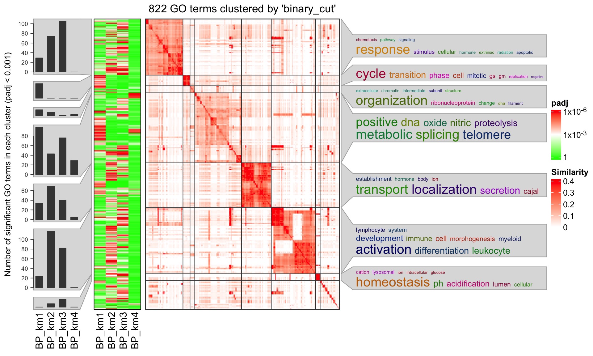
## GO:0006260 278/18614 1.862901e-17 1.474797e-14 1.120682e-14By default, simplifyGOFromMultipleLists() automatically identifies the columns that contain GO IDs and adjusted p-values, so here we directly send lt to simplifyGOFromMultipleLists(). We additionally set padj_cutoff to 0.001 because under the default cutoff 0.01, there are too many GO IDs and to save the running time, we set a more strict cutoff.
simplifyGOFromMultipleLists(lt, padj_cutoff = 0.001)
Next we demonstrate two other data types for simplifyGOFromMultipleLists(). Both usages are straightforward. The first is a list of numeric vectors:
lt2 = lapply(lt, function(x) structure(x$p.adjust, names = x$ID))
simplifyGOFromMultipleLists(lt2, padj_cutoff = 0.001)
And the second is a list of character vectors of GO IDs:
lt3 = lapply(lt, function(x) x$ID[x$p.adjust < 0.001])
simplifyGOFromMultipleLists(lt3)
The process of this analysis is as follows. Let’s assume there are \(n\) GO lists, we first construct a global matrix where columns correspond to the \(n\) GO lists and rows correspond to the “union” of all GO IDs in the \(n\) lists. The value for the ith GO ID and in the jth list are taken from the corresponding numeric vector in lt. If the jth vector in lt does not contain the ith GO ID, the value defined by default argument is taken there (e.g. in most cases the numeric values are adjusted p-values, thus default is set to 1). Let’s call this matrix as \(M_0\).
Next step is to filter \(M_0\) so that we only take a subset of GO IDs of interest. We define a proper function via argument filter to remove GO IDs that are not important for the analysis. Function for filter is applied to every row in \(M_0\) and filter function needs to return a logical value to decide whether to keep or remove the current GO ID. For example, if the values in lt are adjusted p-values, the filter function can be set as function(x) any(x < padj_cutoff) so that the GO ID is kept as long as it is signfiicant in at least one list. After the filtering, let’s call the filtered matrix \(M_1\).
GO IDs in \(M_1\) (row names of \(M_1\)) are used for clustering. A heatmap of \(M_1\) is attached to the left of the GO similarity heatmap so that the group-specific (or list-specific) patterns can be easily observed and to corresponded to GO functions.
Argument heatmap_param controls several parameters for heatmap \(M_1\):
-
transform: A self-defined function to transform the data for heatmap visualization. The most typical case is to transform adjusted p-values by-log10(x). -
breaks: Break values for color interpolation. -
col: The corresponding values forbreaks. -
labels: The corresponding labels for legend. -
name: Legend title.
Session Info
## R version 4.3.3 (2024-02-29)
## Platform: x86_64-apple-darwin20 (64-bit)
## Running under: macOS Sonoma 14.6.1
##
## Matrix products: default
## BLAS:   /Library/Frameworks/R.framework/Versions/4.3-x86_64/Resources/lib/libRblas.0.dylib
## LAPACK: /Library/Frameworks/R.framework/Versions/4.3-x86_64/Resources/lib/libRlapack.dylib;  LAPACK version 3.11.0
##
## Random number generation:
##  RNG:     L'Ecuyer-CMRG
##  Normal:  Inversion
##  Sample:  Rejection
##
## locale:
## [1] en_GB.UTF-8/en_GB.UTF-8/en_GB.UTF-8/C/en_GB.UTF-8/en_GB.UTF-8
##
## time zone: Europe/Berlin
## tzcode source: internal
##
## attached base packages:
## [1] stats4    stats     graphics  grDevices utils     datasets  methods
## [8] base
##
## other attached packages:
##  [1] hu6800.db_3.13.0          org.Hs.eg.db_3.17.0
##  [3] AnnotationDbi_1.62.2      IRanges_2.36.0
##  [5] S4Vectors_0.40.2          Biobase_2.60.0
##  [7] BiocGenerics_0.48.1       cola_2.6.0
##  [9] simplifyEnrichment_1.99.0 knitr_1.45
##
## loaded via a namespace (and not attached):
##   [1] splines_4.3.3           later_1.3.2             ggplotify_0.1.2
##   [4] bitops_1.0-7            tibble_3.2.1            polyclip_1.10-6
##   [7] XML_3.99-0.16.1         lifecycle_1.0.4         doParallel_1.0.17
##  [10] NLP_0.2-1               lattice_0.22-5          prabclus_2.3-3
##  [13] MASS_7.3-60.0.1         magrittr_2.0.3          sass_0.4.9
##  [16] rmarkdown_2.26          jquerylib_0.1.4         yaml_2.3.8
##  [19] httpuv_1.6.15           doRNG_1.8.6             flexmix_2.3-19
##  [22] cowplot_1.1.3           DBI_1.2.2               RColorBrewer_1.1-3
##  [25] eulerr_7.0.2            zlibbioc_1.46.0         expm_0.999-9
##  [28] purrr_1.0.2             ggraph_2.2.1            RCurl_1.98-1.14
##  [31] yulab.utils_0.1.4       nnet_7.3-19             tweenr_2.0.3
##  [34] circlize_0.4.16         GenomeInfoDbData_1.2.10 enrichplot_1.20.3
##  [37] ggrepel_0.9.5           tm_0.7-13               irlba_2.3.5.1
##  [40] tidytree_0.4.6          genefilter_1.82.1       annotate_1.78.0
##  [43] brew_1.0-10             commonmark_1.9.1        pkgdown_2.0.9
##  [46] codetools_0.2-19        ggforce_0.4.2           DOSE_3.26.2
##  [49] xml2_1.3.6              tidyselect_1.2.1        shape_1.4.6.1
##  [52] aplot_0.2.2             farver_2.1.1            viridis_0.6.5
##  [55] matrixStats_1.3.0       dynamicTreeCut_1.63-1   jsonlite_1.8.8
##  [58] GetoptLong_1.0.5        tidygraph_1.3.1         survival_3.5-8
##  [61] iterators_1.0.14        systemfonts_1.0.6       foreach_1.5.2
##  [64] dbscan_1.1-12           tools_4.3.3             treeio_1.24.3
##  [67] ragg_1.3.1              Rcpp_1.0.12             glue_1.7.0
##  [70] gridExtra_2.3           xfun_0.43               qvalue_2.32.0
##  [73] flexclust_1.4-2         MatrixGenerics_1.12.3   GenomeInfoDb_1.36.4
##  [76] dplyr_1.1.4             withr_3.0.0             fastmap_1.1.1
##  [79] fansi_1.0.6             digest_0.6.35           gridGraphics_0.5-1
##  [82] R6_2.5.1                mime_0.12               microbenchmark_1.4.10
##  [85] textshaping_0.3.7       colorspace_2.1-0        GO.db_3.17.0
##  [88] Cairo_1.6-2             markdown_1.12           RSQLite_2.3.6
##  [91] diptest_0.77-1          tidyr_1.3.1             utf8_1.2.4
##  [94] generics_0.1.3          data.table_1.15.4       robustbase_0.99-2
##  [97] class_7.3-22            graphlayouts_1.1.1      httr_1.4.7
## [100] htmlwidgets_1.6.4       scatterpie_0.2.2        scatterplot3d_0.3-44
## [103] MCL_1.0                 pkgconfig_2.0.3         gtable_0.3.5
## [106] modeltools_0.2-23       blob_1.2.4              ComplexHeatmap_2.18.0
## [109] impute_1.74.1           XVector_0.40.0          shadowtext_0.1.3
## [112] clusterProfiler_4.8.3   htmltools_0.5.8.1       fgsea_1.26.0
## [115] clue_0.3-65             scales_1.3.0            png_0.1-8
## [118] ggfun_0.1.4             reshape2_1.4.4          rjson_0.2.21
## [121] nlme_3.1-164            cachem_1.0.8            GlobalOptions_0.1.2
## [124] Polychrome_1.5.1        stringr_1.5.1           parallel_4.3.3
## [127] HDO.db_0.99.1           desc_1.4.3              pillar_1.9.0
## [130] grid_4.3.3              vctrs_0.6.5             slam_0.1-50
## [133] promises_1.3.0          xtable_1.8-4            cluster_2.1.6
## [136] evaluate_0.23           magick_2.8.3            cli_3.6.2
## [139] compiler_4.3.3          rlang_1.1.3             crayon_1.5.2
## [142] rngtools_1.5.2          simona_1.3.12           labeling_0.4.3
## [145] mclust_6.1.1            skmeans_0.2-16          plyr_1.8.9
## [148] fs_1.6.4                stringi_1.8.4           viridisLite_0.4.2
## [151] BiocParallel_1.34.2     munsell_0.5.1           Biostrings_2.68.1
## [154] lazyeval_0.2.2          GOSemSim_2.26.1         Matrix_1.6-5
## [157] patchwork_1.2.0         bit64_4.0.5             ggplot2_3.5.1
## [160] KEGGREST_1.40.1         fpc_2.2-12              shiny_1.8.1.1
## [163] highr_0.10              apcluster_1.4.13        kernlab_0.9-32
## [166] gridtext_0.1.5          igraph_2.0.3            memoise_2.0.1
## [169] bslib_0.7.0             ggtree_3.8.2            fastmatch_1.1-4
## [172] DEoptimR_1.1-3          bit_4.0.5               downloader_0.4
## [175] gson_0.1.0              ape_5.8