7 OncoPrint

OncoPrint is a way to visualize multiple genomic alteration events by heatmap. Here the ComplexHeatmap package provides a oncoPrint() function which makes oncoPrints. Besides the default style which is provided by cBioPortal, there are additional barplots at both sides of the heatmap which show numbers of different alterations for each sample and for each gene. Also with the functionality of ComplexHeatmap, you can concatenate oncoPrints with additional heatmaps and annotations to correspond more types of information.

7.1 General settings

7.1.1 Input data format

There are two different formats of input data. The first is represented as a matrix in which each value can include multiple alterations in a form of a complicated string. In follow example, ‘g1’ in ‘s1’ has two types of alterations which are ‘snv’ and ‘indel.’

mat = read.table(textConnection(
"s1,s2,s3
g1,snv;indel,snv,indel
g2,,snv;indel,snv
g3,snv,,indel;snv"), row.names = 1, header = TRUE, sep = ",", stringsAsFactors = FALSE)
mat = as.matrix(mat)
mat

##    s1          s2          s3         
## g1 "snv;indel" "snv"       "indel"    
## g2 ""          "snv;indel" "snv"      
## g3 "snv"       ""          "indel;snv"

In this case, we need to define a function to extract different alteration types from these long strings. The definition of such function is always simple, it accepts the complicated string and returns a vector of alteration types.

For mat, we can define the function as:

get_type_fun = function(x) strsplit(x, ";")[[1]]
get_type_fun(mat[1, 1])

## [1] "snv"   "indel"

get_type_fun(mat[1, 2])

## [1] "snv"

So, if the alterations are encoded as snv|indel, you can define the function as function(x) strsplit(x, "|")[[1]]. This self-defined function is assigned to the get_type argument in oncoPrint().

Since in most cases, the separators are only single characters, If the separators are in ;:,|, oncoPrint() automatically spit the alteration strings so that you don’t need to explicitely specify get_type in oncoPrint() function.

For one gene in one sample, since different alteration types may be drawn into one same grid in the heatmap, we need to define how to add the graphics by providing a list of self-defined functions to alter_fun argument. Here if the graphics have no transparency, order of adding graphics matters. In following example, snv are first drawn and then the indel. You can see rectangles for indels are actually smaller (0.4*h) than that for snvs (0.9*h) so that you can visualize both snvs and indels if they are in a same grid. Names of the function list should correspond to the alteration types (here, snv and indel).

For the self-defined graphic function (the functions in alter_fun, there should be four arguments which are positions of the grids on the oncoPrint (x and y), and widths and heights of the grids (w and h, which is measured in npc unit). Proper values for the four arguments are sent to these functions automatically from oncoPrint().

Colors for different alterations are defined in col. It should be a named vector for which names correspond to alteration types. It is used to generate the barplots.

col = c(snv = "red", indel = "blue")
oncoPrint(mat,
    alter_fun = list(
        snv = function(x, y, w, h) grid.rect(x, y, w*0.9, h*0.9, 
            gp = gpar(fill = col["snv"], col = NA)),
        indel = function(x, y, w, h) grid.rect(x, y, w*0.9, h*0.4, 
            gp = gpar(fill = col["indel"], col = NA))
    ), col = col)

You can see the order in barplots also correspond to the order defined in alter_fun. The grahpics in legend are based on the functions defined in alter_fun.

If you are confused of how to generated the matrix, there is a second way. The second type of input data is a list of matrix for which each matrix contains binary value representing whether the alteration is absent or present. The list should have names which correspond to the alteration types.

mat_list = list(snv = matrix(c(1, 0, 1, 1, 1, 0, 0, 1, 1), nrow = 3),
                indel = matrix(c(1, 0, 0, 0, 1, 0, 1, 0, 0), nrow = 3))
rownames(mat_list$snv) = rownames(mat_list$indel) = c("g1", "g2", "g3")
colnames(mat_list$snv) = colnames(mat_list$indel) = c("s1", "s2", "s3")
mat_list

## $snv
##    s1 s2 s3
## g1  1  1  0
## g2  0  1  1
## g3  1  0  1
## 
## $indel
##    s1 s2 s3
## g1  1  0  1
## g2  0  1  0
## g3  0  0  0

oncoPrint() expects all matrices in mat_list having same row names and column names.

Pass mat_list to oncoPrint():

# now you don't need `get_type`
oncoPrint(mat_list,
    alter_fun = list(
        snv = function(x, y, w, h) grid.rect(x, y, w*0.9, h*0.9, 
            gp = gpar(fill = col["snv"], col = NA)),
        indel = function(x, y, w, h) grid.rect(x, y, w*0.9, h*0.4, 
            gp = gpar(fill = col["indel"], col = NA))
    ), col = col)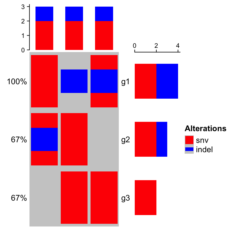

In following parts of this chapter, we still use the single matrix form mat to specify the input data.

7.1.2 Define the alter_fun()

alter_fun is a list of functons which add graphics layer by layer (i.e. first draw for snv, then for indel). Graphics can also be added in a grid-by-grid style by specifying alter_fun as a single function. The difference from the function list is now alter_fun should accept a fifth argument which is a logical vector. This logical vector shows whether different alterations exist for current gene in current sample.

Let’s assume in a grid there is only snv event, then v for this grid is:

##   snv indel 
##  TRUE FALSE

oncoPrint(mat,
    alter_fun = function(x, y, w, h, v) {
        if(v["snv"]) grid.rect(x, y, w*0.9, h*0.9, # v["snv"] is a logical value
            gp = gpar(fill = col["snv"], col = NA))
        if(v["indel"]) grid.rect(x, y, w*0.9, h*0.4, # v["indel"] is a logical value
            gp = gpar(fill = col["indel"], col = NA))
    }, col = col)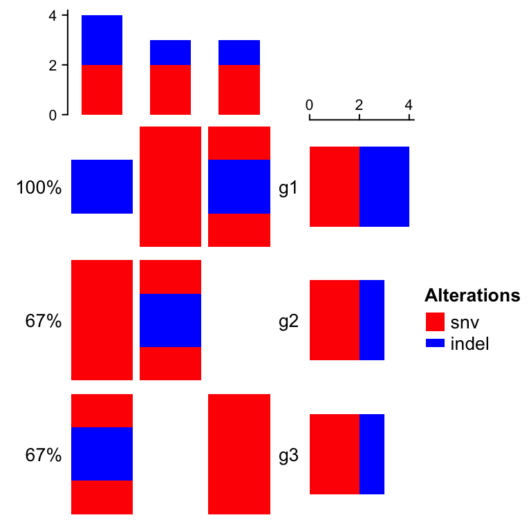

If alter_fun is set as a single function, customization can be more flexible. In following example, the blue rectangles can have different height in different grid.

oncoPrint(mat,
    alter_fun = function(x, y, w, h, v) {
        n = sum(v)  # how many alterations for current gene in current sample
        h = h*0.9
        # use `names(which(v))` to correctly map between `v` and `col`
        if(n) grid.rect(x, y - h*0.5 + 1:n/n*h, w*0.9, 1/n*h, 
            gp = gpar(fill = col[names(which(v))], col = NA), just = "top")
    }, col = col)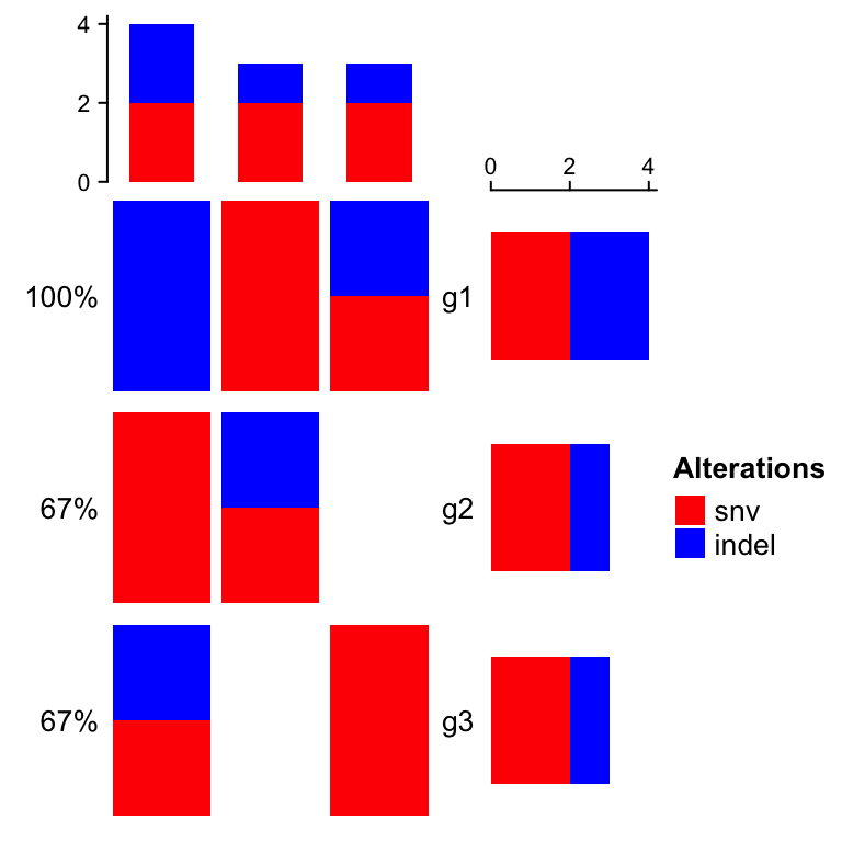

Following is a complicated example for alter_fun where triangles are used:

oncoPrint(mat,
    alter_fun = list(
        background = function(x, y, w, h) {
            grid.polygon(
                unit.c(x - 0.5*w, x - 0.5*w, x + 0.5*w), 
                unit.c(y - 0.5*h, y + 0.5*h, y - 0.5*h),
                gp = gpar(fill = "grey", col = "white"))
            grid.polygon(
                unit.c(x + 0.5*w, x + 0.5*w, x - 0.5*w), 
                unit.c(y + 0.5*h, y - 0.5*h, y + 0.5*h),
                gp = gpar(fill = "grey", col = "white"))
        },
        snv = function(x, y, w, h) {
            grid.polygon(
                unit.c(x - 0.5*w, x - 0.5*w, x + 0.5*w), 
                unit.c(y - 0.5*h, y + 0.5*h, y - 0.5*h),
                gp = gpar(fill = col["snv"], col = "white"))
        },
        indel = function(x, y, w, h) {
            grid.polygon(
                unit.c(x + 0.5*w, x + 0.5*w, x - 0.5*w), 
                unit.c(y + 0.5*h, y - 0.5*h, y + 0.5*h),
                gp = gpar(fill = col["indel"], col = "white"))
        }
    ), col = col)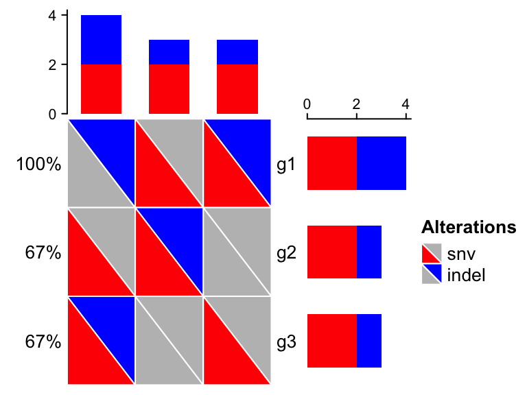

In some cases, you might need to define alter_fun for many alteration types. If you are not sure about the visual effect of your alter_fun, you can use test_alter_fun() to test your alter_fun. In following example, we defined seven alteration functions:

alter_fun = list(
    mut1 = function(x, y, w, h) 
        grid.rect(x, y, w, h, gp = gpar(fill = "red", col = NA)),
    mut2 = function(x, y, w, h) 
        grid.rect(x, y, w, h, gp = gpar(fill = "blue", col = NA)),
    mut3 = function(x, y, w, h) 
        grid.rect(x, y, w, h, gp = gpar(fill = "yellow", col = NA)),
    mut4 = function(x, y, w, h) 
        grid.rect(x, y, w, h, gp = gpar(fill = "purple", col = NA)),
    mut5 = function(x, y, w, h) 
        grid.rect(x, y, w, h, gp = gpar(fill = NA, lwd = 2)),
    mut6 = function(x, y, w, h) 
        grid.points(x, y, pch = 16),
    mut7 = function(x, y, w, h) 
        grid.segments(x - w*0.5, y - h*0.5, x + w*0.5, y + h*0.5, gp = gpar(lwd = 2))
)
test_alter_fun(alter_fun)

## `alter_fun` is defined as a list of functions.
## Functions are defined for following alteration types:
##   mut1, mut2, mut3, mut4, mut5, mut6, mut7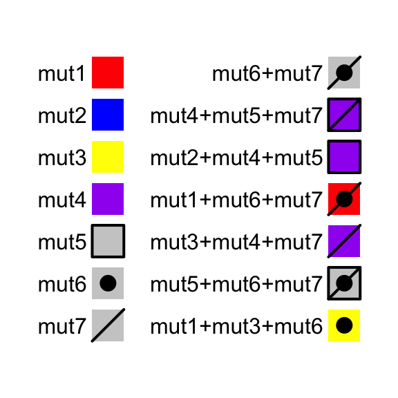

For the combination of alteration types, test_alter_fun() randomly samples some of them.

test_alter_fun() works both for alter_fun as a list and as a single function.

7.1.3 Background

If alter_fun is specified as a list, the order of the elements controls the order of adding graphics. There is a special element called background which defines how to draw background and it should be always put as the first element in the alter_fun list. In following example, backgrond color is changed to light green with borders.

oncoPrint(mat,
    alter_fun = list(
        background = function(x, y, w, h) grid.rect(x, y, w, h, 
            gp = gpar(fill = "#00FF0020")),
        snv = function(x, y, w, h) grid.rect(x, y, w*0.9, h*0.9, 
            gp = gpar(fill = col["snv"], col = NA)),
        indel = function(x, y, w, h) grid.rect(x, y, w*0.9, h*0.4, 
            gp = gpar(fill = col["indel"], col = NA))
    ), col = col)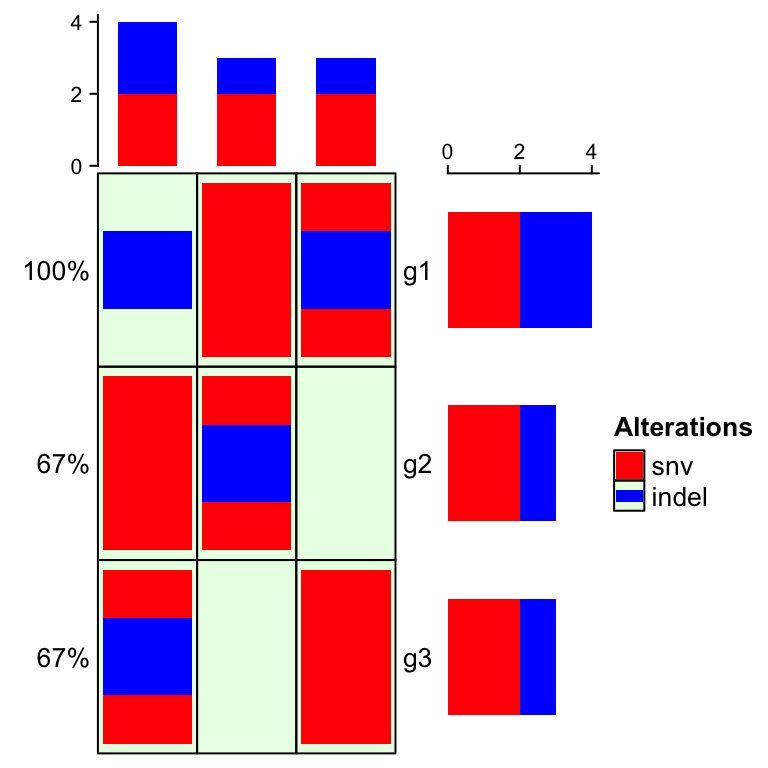

Or just remove the background (don’t set it to NULL. Setting background directly to NULL means to use the default style of background whch is in grey):

oncoPrint(mat,
    alter_fun = list(
        background = function(...) NULL,
        snv = function(x, y, w, h) grid.rect(x, y, w*0.9, h*0.9, 
            gp = gpar(fill = col["snv"], col = NA)),
        indel = function(x, y, w, h) grid.rect(x, y, w*0.9, h*0.4, 
            gp = gpar(fill = col["indel"], col = NA))
    ), col = col)

7.1.4 Complex alteration types

It is very easy to have many more different alteration types when integrating information from multiple analysis results. It is sometimes difficult to design graphics and assign different colors for them (e.g. see plot in this link. On the other hand, in these alteration types, there are primary classes of alteration types which is more important to distinguish, while there are secondary classes which is less important. For example, we may have alteration types of “intronic snv,” “exonic snv,” “intronic indel” and “exonic indel.” Actually we can classify them into two classes where “snv/indel” is more important and they belong to the primary class, and “intronic/exonic” is less important and they belong to the secondary class. Reflecting on the oncoPrint, for the “intronic snv” and “exonic snv,” we want to use similar graphics because they are snvs and we want them visually similar, and we add slightly different symbols to represent “intronic” and “exonic,” E.g. we can use red rectangle for snv and above the red rectangles, we use dots to represent “intronic” and cross lines to represent “exonic.” On the barplot annotations which summarize the number of different alteration types, we don’t want to separate “intronic snv” and “exonic snv” while we prefer to simply get the total number of snv to get rid of too many categories in the barplots.

Let’s demonstrate this scenario by following simulated data. To simplify the example, we assume for a single gene in a single sample, it only has either snv or indel and it can only be either intronic or exonic. If there is no “intronic” or “exonic” attached to the gene, it basically means we don’t have this gene-related information (maybe it is an intergenic snv/indel).

set.seed(123)
x1 = sample(c("", "snv"), 100, replace = TRUE, prob = c(8, 2))
x2 = sample(c("", "indel"), 100, replace = TRUE, prob = c(8, 2))
x2[x1 == "snv"] = ""
x3 = sample(c("", "intronic"), 100, replace = TRUE, prob = c(5, 5))
x4 = sample(c("", "exonic"), 100, replace = TRUE, prob = c(5, 5))
x3[x1 == "" & x2 == ""] = ""
x4[x1 == "" & x2 == ""] = ""
x4[x3 == "intronic"] = ""
x = apply(cbind(x1, x2, x3, x4), 1, function(x) {
    x = x[x != ""]
    paste(x, collapse = ";")
})
m = matrix(x, nrow = 10, ncol = 10, dimnames = list(paste0("g", 1:10), paste0("s", 1:10)))
m[1:4, 1:4]

##    s1    s2             s3             s4            
## g1 ""    "snv;intronic" "snv;intronic" "snv"         
## g2 ""    ""             ""             "snv;intronic"
## g3 ""    ""             ""             ""            
## g4 "snv" "indel;exonic" "snv"          ""

Now in m, there are four different alteration types: snv, indel, intronic and exonic. Next we define alter_fun for the four alterations.

alter_fun = list(
    background = function(x, y, w, h) 
        grid.rect(x, y, w*0.9, h*0.9, gp = gpar(fill = "#CCCCCC", col = NA)),
    # red rectangles
    snv = function(x, y, w, h) 
        grid.rect(x, y, w*0.9, h*0.9, gp = gpar(fill = "red", col = NA)),
    # blue rectangles
    indel = function(x, y, w, h) 
        grid.rect(x, y, w*0.9, h*0.9, gp = gpar(fill = "blue", col = NA)),
    # dots
    intronic = function(x, y, w, h) 
        grid.points(x, y, pch = 16),
    # crossed lines
    exonic = function(x, y, w, h) {
        grid.segments(x - w*0.4, y - h*0.4, x + w*0.4, y + h*0.4, gp = gpar(lwd = 2))
        grid.segments(x + w*0.4, y - h*0.4, x - w*0.4, y + h*0.4, gp = gpar(lwd = 2))
    }
)

For the alteration types in the primary class (snv and indel), we use colorred rectangles to represent them because the rectangles are visually obvious, while for the alteration types in the secondary class (intronic and exonic), we only use simple symbols (dots for intronic and crossed diagonal lines for exonic). Since there is no color corresponding to intronic and exonic, we don’t need to define colors for these two types, and on the barplot annotation for genes and samples, only snv and indel are visualized (so the height for snv in the barplot corresponds the number of intronic snv plus exonic snv).

# we only define color for snv and indel, so barplot annotations only show snv and indel
oncoPrint(m, alter_fun = alter_fun, col = c(snv = "red", indel = "blue"))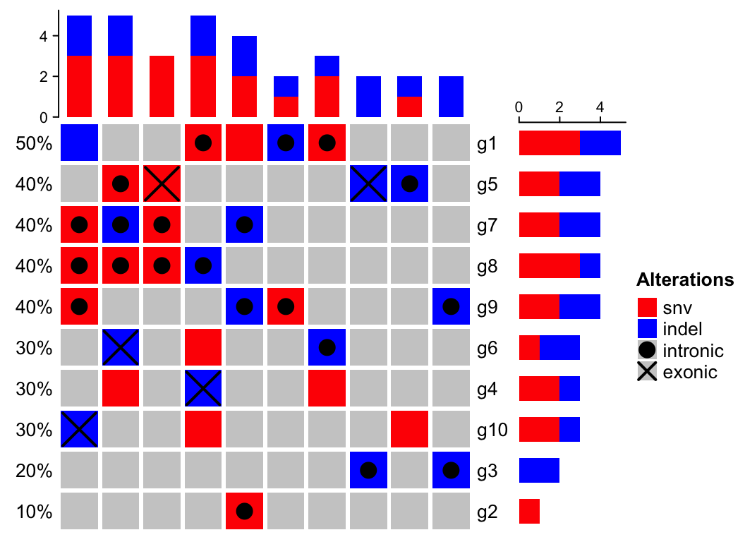

7.1.5 Simplify alter_fun

If the graphics are only simple graphics, e.g., rectangles, points, the graphic functions can be automatically generated by alter_graphic() function. One of previous example can be simplied as:

oncoPrint(mat,
    alter_fun = list(
        snv = alter_graphic("rect", width = 0.9, height = 0.9, fill = col["snv"]),
        indel = alter_graphic("rect", width = 0.9, height = 0.4, fill = col["indel"])
    ), col = col)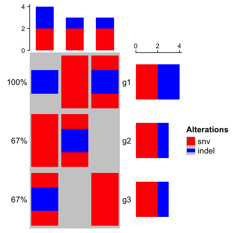

7.1.6 Other heatmap-related settings

Column names are by default not drawn in the plot. It is can be turned on by setting show_column_names = TRUE.

alter_fun = list(
    snv = function(x, y, w, h) grid.rect(x, y, w*0.9, h*0.9, 
        gp = gpar(fill = col["snv"], col = NA)),
    indel = function(x, y, w, h) grid.rect(x, y, w*0.9, h*0.4, 
        gp = gpar(fill = col["indel"], col = NA))
)
oncoPrint(mat, alter_fun = alter_fun, col = col, show_column_names = TRUE)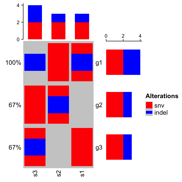

Row names and percent texts can be turned on/off by setting show_pct and show_row_names. The side of both according to the oncoPrint is controlled by pct_side and row_names_side. Digits of the percent values are controlled by pct_digits.

oncoPrint(mat, alter_fun = alter_fun, col = col, 
    row_names_side = "left", pct_side = "right", pct_digits = 2)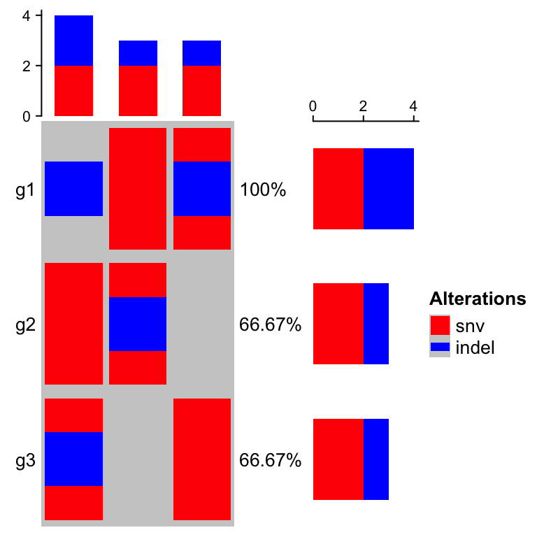

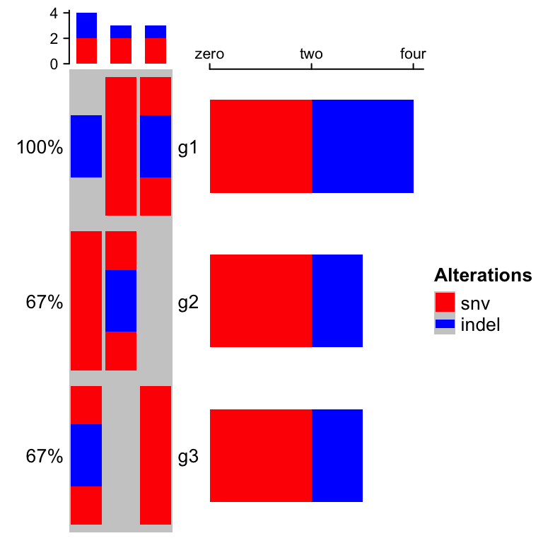
The barplot annotations on the both side are controlled by anno_oncoprint_barplot() annotation function. Customization such as the size and the axes can be set directly in anno_oncoprint_barplot(). More examples of setting anno_oncoprint_barplot() can be found in Section 7.2.3.

oncoPrint(mat, alter_fun = alter_fun, col = col, 
    top_annotation = HeatmapAnnotation(
        cbar = anno_oncoprint_barplot(height = unit(1, "cm"))),
    right_annotation = rowAnnotation(
        rbar = anno_oncoprint_barplot(
            width = unit(4, "cm"),
            axis_param = list(at = c(0, 2, 4), 
                labels = c("zero", "two", "four"),
                side = "top",
                labels_rot = 0))),
    )

Some people might want to move the right barplots to the left of the oncoPrint:

oncoPrint(mat, alter_fun = alter_fun, col = col, 
    left_annotation =  rowAnnotation(
        rbar = anno_oncoprint_barplot(
            axis_param = list(direction = "reverse")
    )),
    right_annotation = NULL)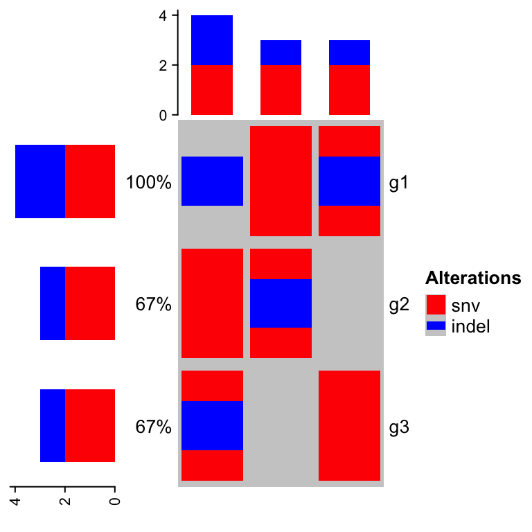

OncoPrints essentially are heatmaps, thus, there are many arguments set in Heatmap() can also be set in oncoPrint(). In following section, we use a real-world dataset to demonstrate more use of oncoPrint() function.

7.2 Apply to cBioPortal dataset

We use a real-world dataset to demonstrate advanced usage of oncoPrint(). The data is retrieved from cBioPortal. Steps for getting the data are as follows:

1. go to http://www.cbioportal.org,
2. search Cancer Study: “Lung Adenocarcinoma Carcinoma” and select: “Lung Adenocarcinoma Carcinoma (TCGA, Provisinal),”
3. in “Enter Gene Set” field, select: “General: Ras-Raf-MEK-Erk/JNK signaling (26 genes),”
4. submit the form.

In the result page,

5. go to “Download” tab, download text in “Type of Genetic alterations across all cases.”

The order of samples can also be downloaded from the results page,

6. go to “OncoPrint” tab, move the mouse above the plot, click “download” icon and click “Sample order.”

The data is already in ComplexHeatmap package. First we read the data and make some pre-processing.

mat = read.table(system.file("extdata", package = "ComplexHeatmap", 
    "tcga_lung_adenocarcinoma_provisional_ras_raf_mek_jnk_signalling.txt"), 
    header = TRUE, stringsAsFactors = FALSE, sep = "\t")
mat[is.na(mat)] = ""
rownames(mat) = mat[, 1]
mat = mat[, -1]
mat=  mat[, -ncol(mat)]
mat = t(as.matrix(mat))
mat[1:3, 1:3]

##      TCGA-05-4384-01 TCGA-05-4390-01 TCGA-05-4425-01
## KRAS "  "            "MUT;"          "  "           
## HRAS "  "            "  "            "  "           
## BRAF "  "            "  "            "  "

There are three different alterations in mat: HOMDEL, AMP and MUT. We first define how to add graphics for different alterations.

col = c("HOMDEL" = "blue", "AMP" = "red", "MUT" = "#008000")
alter_fun = list(
    background = function(x, y, w, h) {
        grid.rect(x, y, w-unit(2, "pt"), h-unit(2, "pt"), 
            gp = gpar(fill = "#CCCCCC", col = NA))
    },
    # big blue
    HOMDEL = function(x, y, w, h) {
        grid.rect(x, y, w-unit(2, "pt"), h-unit(2, "pt"), 
            gp = gpar(fill = col["HOMDEL"], col = NA))
    },
    # big red
    AMP = function(x, y, w, h) {
        grid.rect(x, y, w-unit(2, "pt"), h-unit(2, "pt"), 
            gp = gpar(fill = col["AMP"], col = NA))
    },
    # small green
    MUT = function(x, y, w, h) {
        grid.rect(x, y, w-unit(2, "pt"), h*0.33, 
            gp = gpar(fill = col["MUT"], col = NA))
    }
)

Just a note, since the graphics are all rectangles, they can be simplied by generating by alter_graphic():

# just for demonstration
alter_fun = list(
    background = alter_graphic("rect", fill = "#CCCCCC"),   
    HOMDEL = alter_graphic("rect", fill = col["HOMDEL"]),
    AMP = alter_graphic("rect", fill = col["AMP"]),
    MUT = alter_graphic("rect", height = 0.33, fill = col["MUT"])
)

Now we make the oncoPrint. We save column_title and heatmap_legend_param as varaibles because they are used multiple times in following code chunks.

column_title = "OncoPrint for TCGA Lung Adenocarcinoma, genes in Ras Raf MEK JNK signalling"
heatmap_legend_param = list(title = "Alternations", at = c("HOMDEL", "AMP", "MUT"), 
        labels = c("Deep deletion", "Amplification", "Mutation"))
oncoPrint(mat,
    alter_fun = alter_fun, col = col, 
    column_title = column_title, heatmap_legend_param = heatmap_legend_param)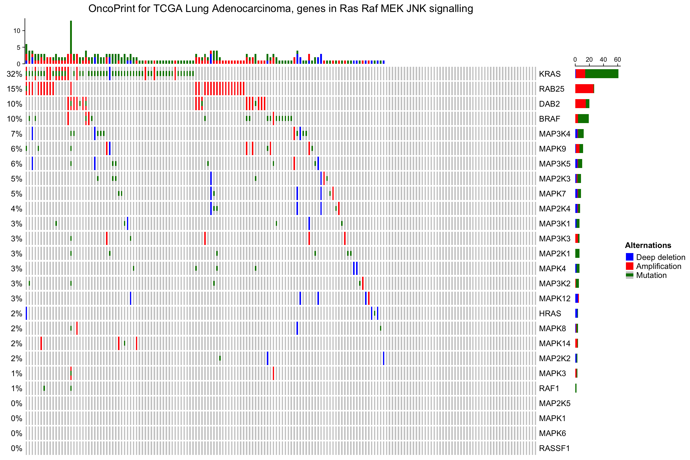

As you see, the genes and samples are reordered automatically. Rows are sorted based on the frequency of the alterations in all samples and columns are reordered to visualize the mutual exclusivity between samples. The column reordering is based on the “memo sort” method, adapted from https://gist.github.com/armish/564a65ab874a770e2c26.

7.2.1 Remove empty rows and columns

By default, if samples or genes have no alterations, they will still remain in the heatmap, but you can set remove_empty_columns and remove_empty_rows to TRUE to remove them:

oncoPrint(mat,
    alter_fun = alter_fun, col = col, 
    remove_empty_columns = TRUE, remove_empty_rows = TRUE,
    column_title = column_title, heatmap_legend_param = heatmap_legend_param)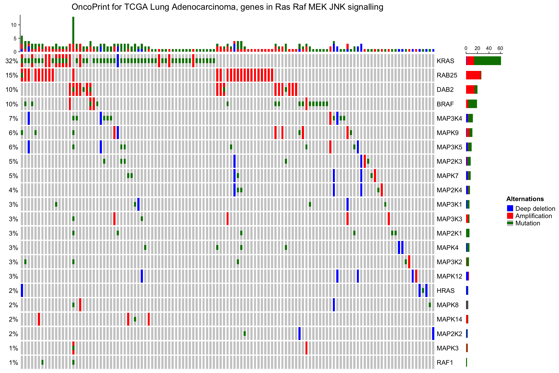

The number of rows and columns may be reduced after empty rows and columns are removed. All the components of the oncoPrint are adjusted accordingly. When the oncoPrint is concatenated with other heatmaps and annotations, this may cause a problem that the number of rows or columns are not all identical in the heatmap list. So, if you put oncoPrint into a heatmap list and you don’t want to see empty rows or columns, you need to remove them manually before sending to oncoPrint() function (this preprocess should be very easy for you!).

7.2.2 Reorder the oncoPrint

As the normal Heatmap() function, row_order or column_order can be assigned with a vector of orders (either numeric or character). In following example, the order of samples are gathered from cBio as well. You can see the difference for the sample order between ‘memo sort’ and the method used by cBio.

sample_order = scan(paste0(system.file("extdata", package = "ComplexHeatmap"), 
    "/sample_order.txt"), what = "character")
oncoPrint(mat,
    alter_fun = alter_fun, col = col, 
    row_order = 1:nrow(mat), column_order = sample_order,
    remove_empty_columns = TRUE, remove_empty_rows = TRUE,
    column_title = column_title, heatmap_legend_param = heatmap_legend_param)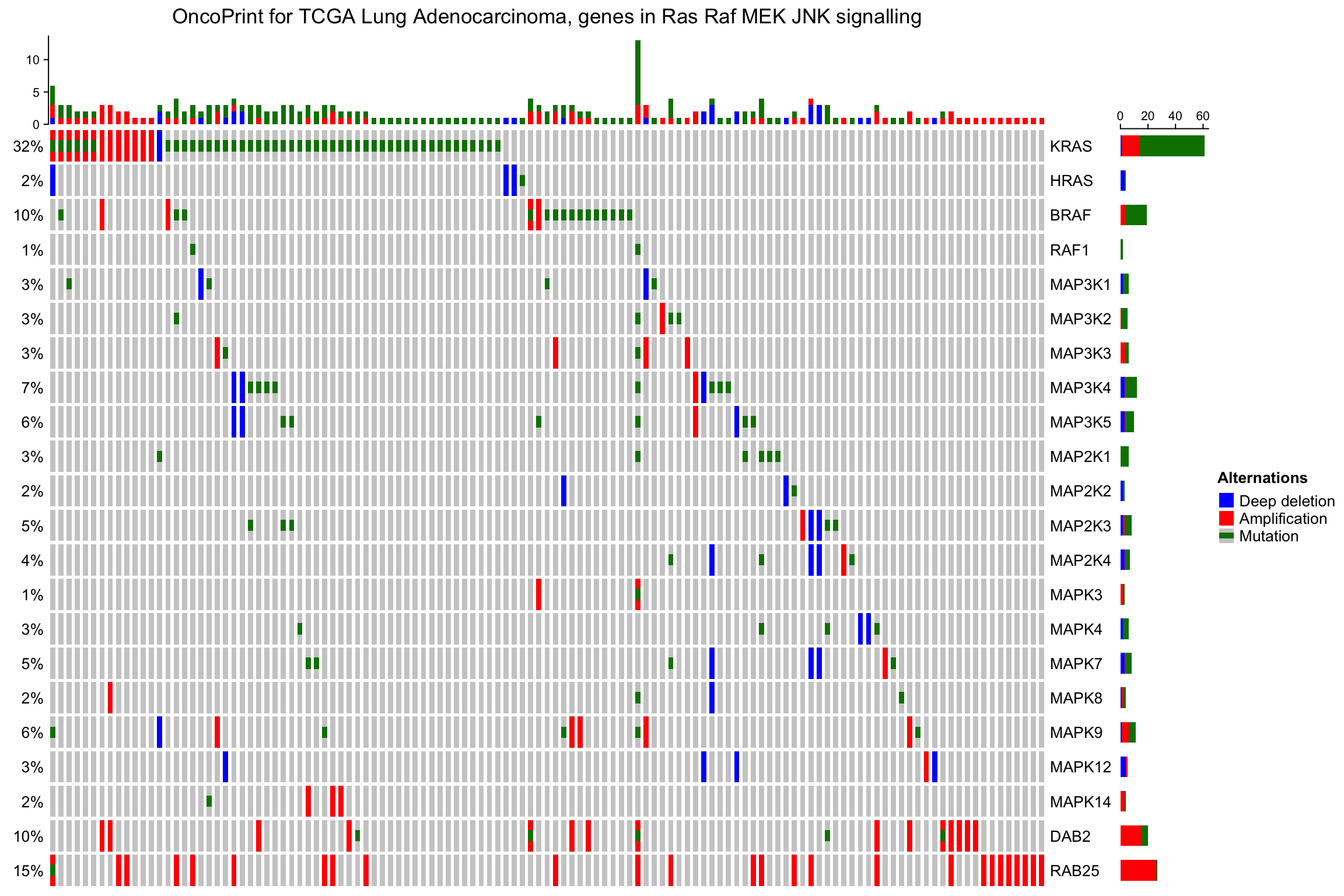

Again, row_order and column_order are automatically adjusted if remove_empty_rows and remove_empty_columns are set to TRUE.

7.2.3 OncoPrint annotations

The oncoPrint has several pre-defined annotations.

On top and right of the oncoPrint, there are barplots showing the number of different alterations for each gene or for each sample, and on the left of the oncoPrint is a text annotation showing the percent of samples that have alterations for every gene.

The barplot annotation is implemented by anno_oncoprint_barplot() where you can set the the annotation there. Barplots by default draw for all alteration types, but you can also select subset of alterations to put on barplots by setting in anno_oncoprint_barplot(). anno_oncoprint_barplot() is a simple wrapper around anno_barplot() where the frequency matrix in just interanlly calculated. See following example:

oncoPrint(mat,
    alter_fun = alter_fun, col = col, 
    top_annotation = HeatmapAnnotation(
        column_barplot = anno_oncoprint_barplot("MUT", border = TRUE, # only MUT
            height = unit(4, "cm"))
    ),
    right_annotation = rowAnnotation(
        row_barplot = anno_oncoprint_barplot(c("AMP", "HOMDEL"),  # only AMP and HOMDEL
            border = TRUE, height = unit(4, "cm"), 
            axis_param = list(side = "bottom", labels_rot = 90))
    ),
    remove_empty_columns = TRUE, remove_empty_rows = TRUE,
    column_title = column_title, heatmap_legend_param = heatmap_legend_param)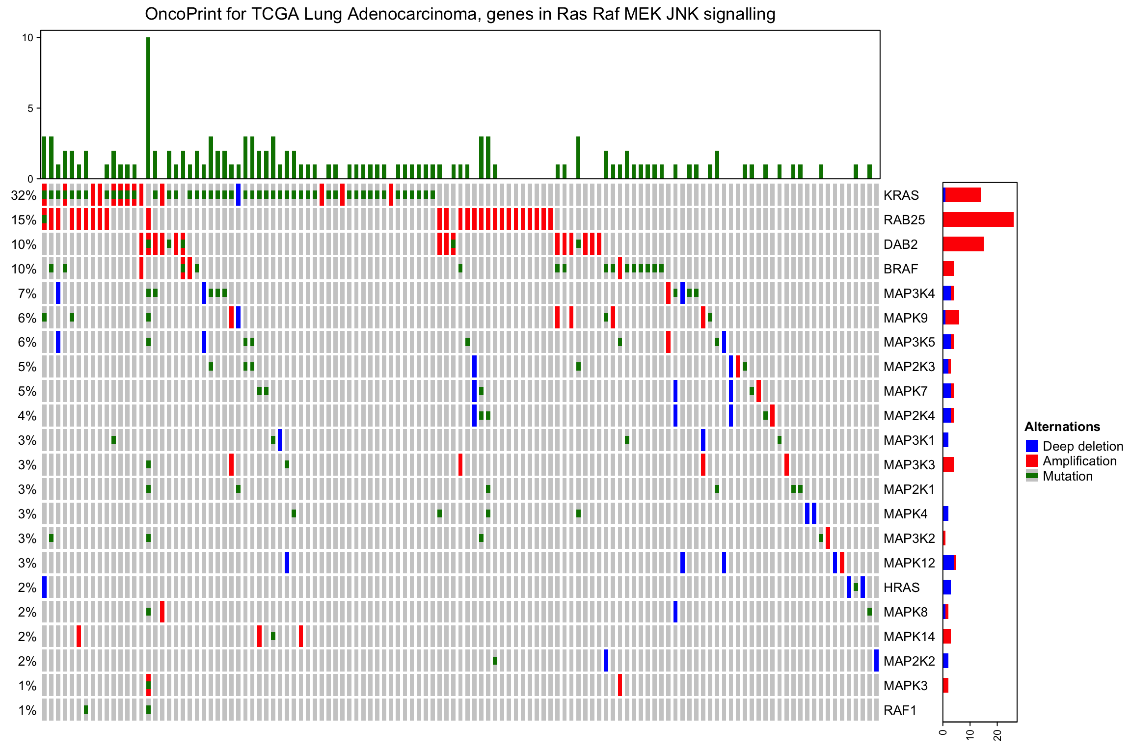

By default the barplot annotation shows the frequencies. The values can be changed to fraction by setting show_fraction = TRUE in anno_oncoprint_barplot():

oncoPrint(mat,
    alter_fun = alter_fun, col = col, 
    top_annotation = HeatmapAnnotation(
        column_barplot = anno_oncoprint_barplot(show_fraction = TRUE)
    ),
    right_annotation = rowAnnotation(
        row_barplot = anno_oncoprint_barplot(show_fraction = TRUE)
    ),
    remove_empty_columns = TRUE, remove_empty_rows = TRUE,
    column_title = column_title, heatmap_legend_param = heatmap_legend_param)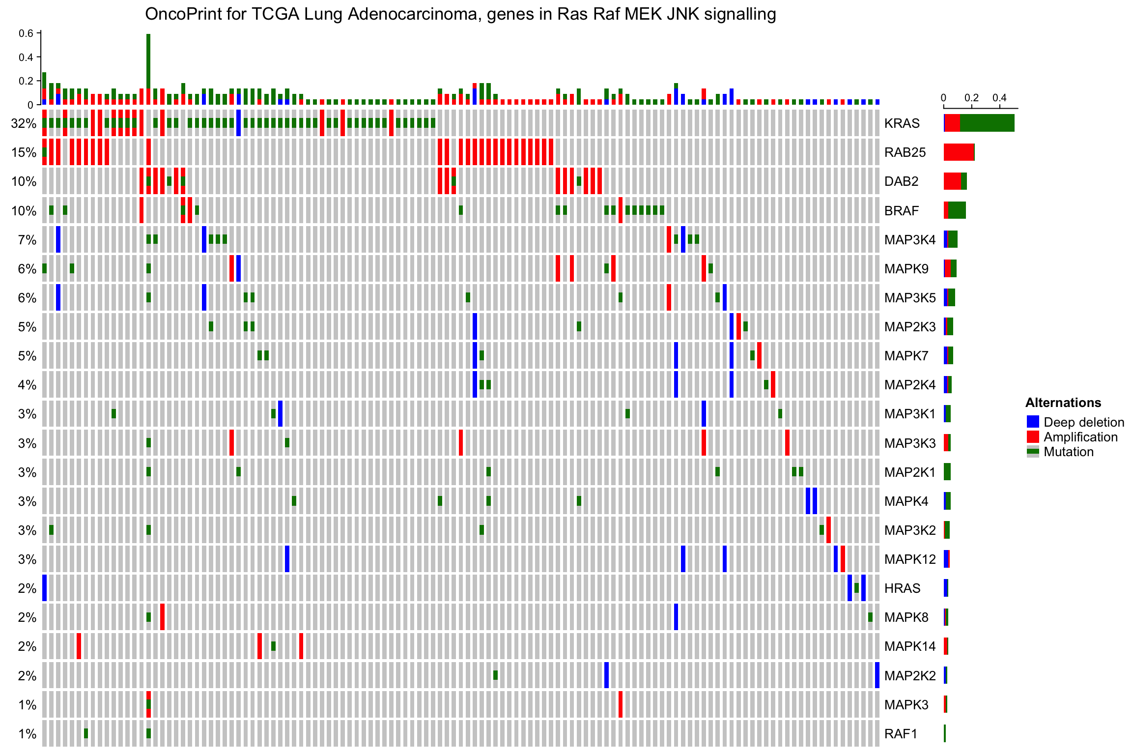

The percent values and row names are internally constructed as text annotations. You can set show_pct and show_row_names to turn them on or off. pct_side and row_names_side controls the sides where they are put.

oncoPrint(mat,
    alter_fun = alter_fun, col = col, 
    remove_empty_columns = TRUE, remove_empty_rows = TRUE,
    pct_side = "right", row_names_side = "left",
    column_title = column_title, heatmap_legend_param = heatmap_legend_param)

The barplot annotation for oncoPrint are essentially normal annotations, you can add more annotations in HeatmapAnnotation() or rowAnnotation() in the normal way:

oncoPrint(mat,
    alter_fun = alter_fun, col = col, 
    remove_empty_columns = TRUE, remove_empty_rows = TRUE,
    top_annotation = HeatmapAnnotation(cbar = anno_oncoprint_barplot(),
        foo1 = 1:172,
        bar1 = anno_points(1:172)
    ),
    left_annotation = rowAnnotation(foo2 = 1:26),
    right_annotation = rowAnnotation(bar2 = anno_barplot(1:26)),
    column_title = column_title, heatmap_legend_param = heatmap_legend_param)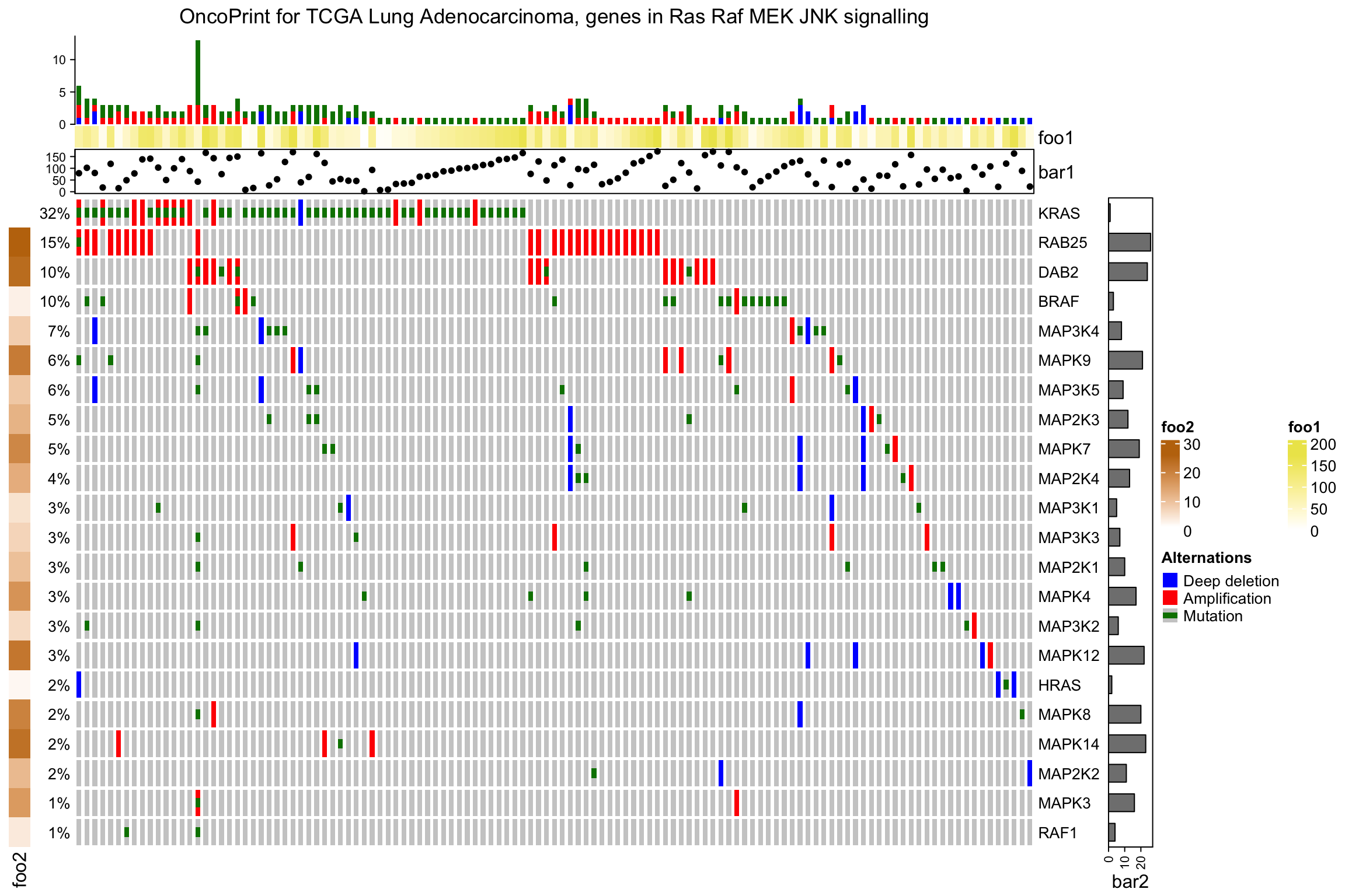

As you see, the percent annotation, the row name annotation and the oncoPrint annotation are appended to the user-specified annotation by default. Also annotations are automatically adjusted if remove_empty_columns and remove_empty_rows are set to TRUE.

7.2.4 oncoPrint as a Heatmap

oncoPrint() actually returns a Heatmap object, so you can add more heatmaps and annotations horizontally or vertically to visualize more complicated associations.

Following example adds a heatmap horizontally. Remember you can always add row annotations to the heatmap list.

ht_list = oncoPrint(mat,
    alter_fun = alter_fun, col = col, 
    column_title = column_title, heatmap_legend_param = heatmap_legend_param) +
Heatmap(matrix(rnorm(nrow(mat)*10), ncol = 10), name = "expr", width = unit(4, "cm"))
draw(ht_list)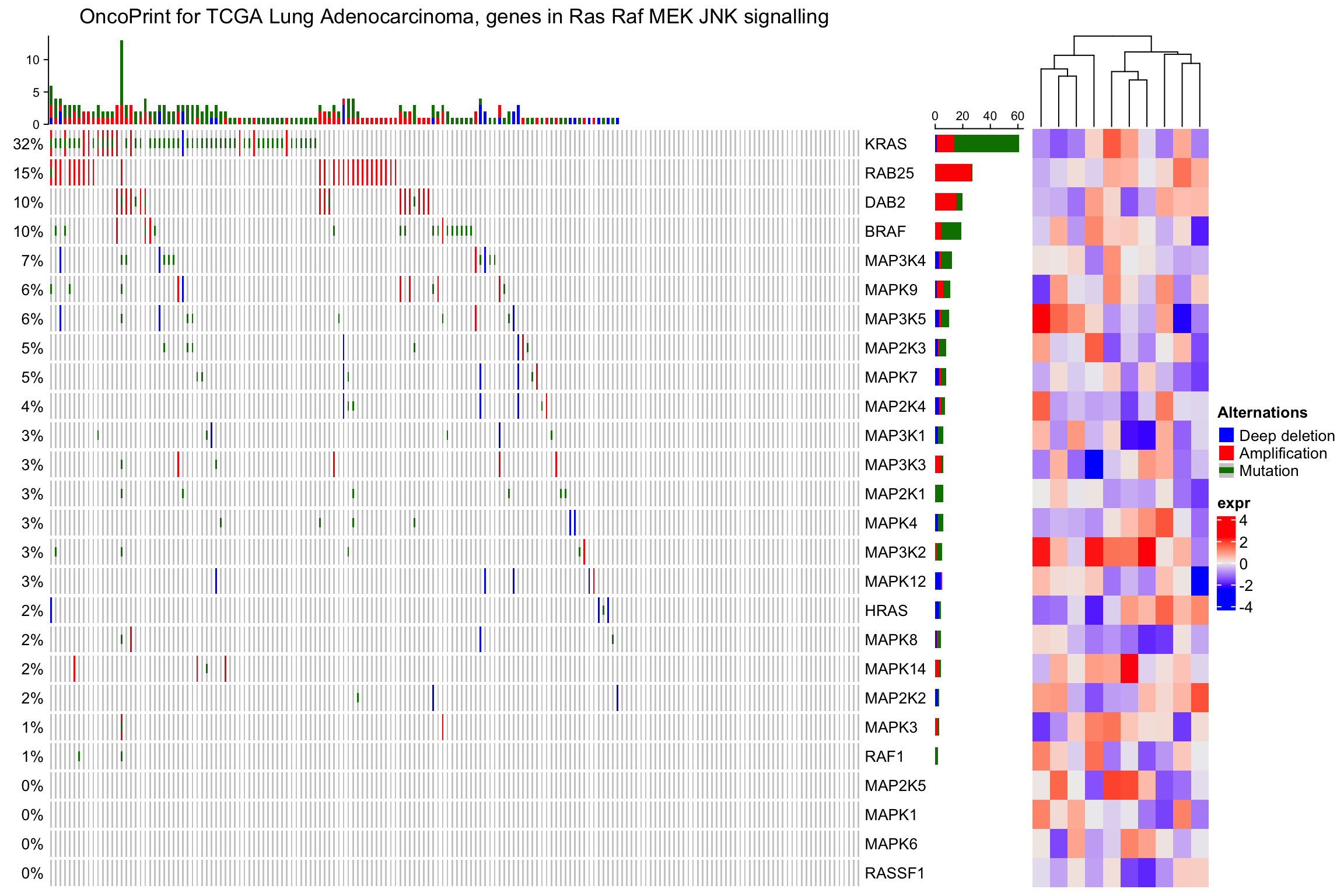

or add it vertically:

ht_list = oncoPrint(mat,
    alter_fun = alter_fun, col = col, 
    column_title = column_title, heatmap_legend_param = heatmap_legend_param) %v%
Heatmap(matrix(rnorm(ncol(mat)*10), nrow = 10), name = "expr", height = unit(4, "cm"))
draw(ht_list)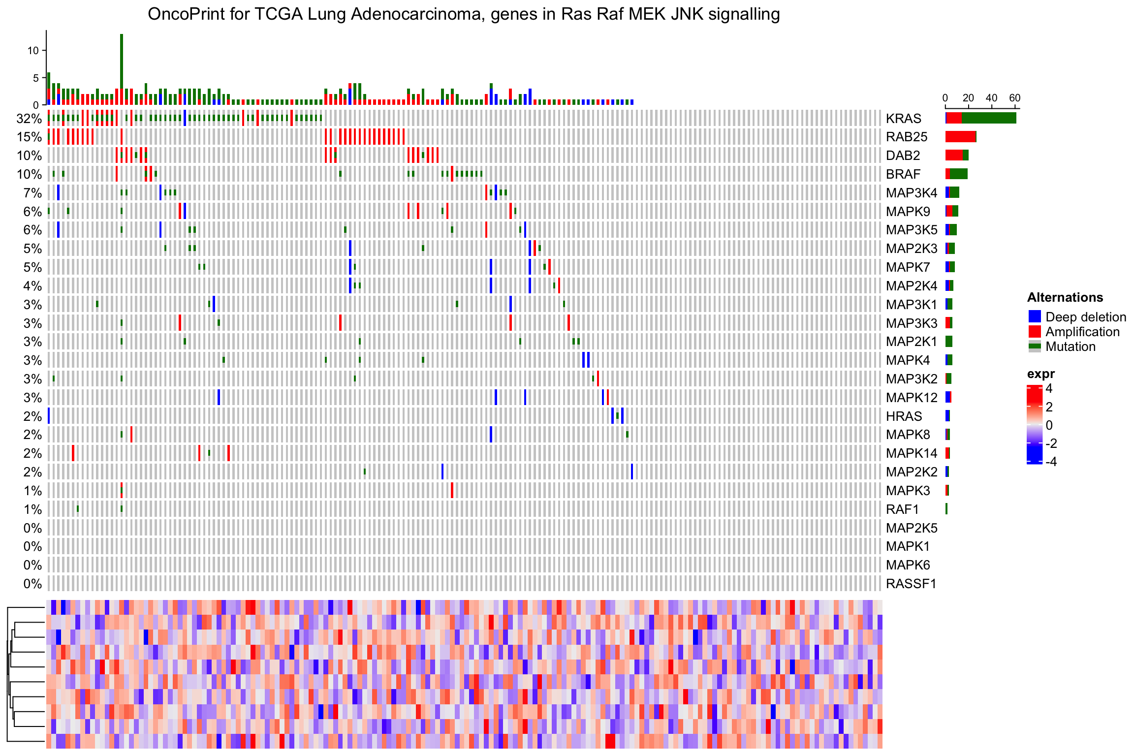

Similar as normal heatmap list, you can split the heatmap list:

ht_list = oncoPrint(mat,
    alter_fun = alter_fun, col = col, 
    column_title = column_title, heatmap_legend_param = heatmap_legend_param) +
Heatmap(matrix(rnorm(nrow(mat)*10), ncol = 10), name = "expr", width = unit(4, "cm"))
draw(ht_list, row_split = sample(c("a", "b"), nrow(mat), replace = TRUE))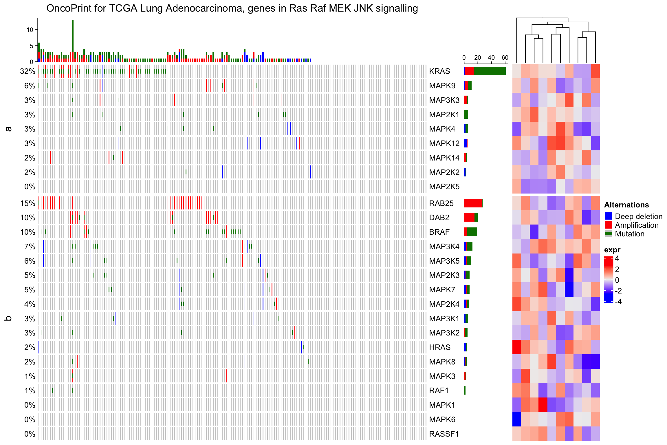

When remove_empty_columns or remove_empty_rows is set to TRUE, the number of genes or the samples may not be the original number. If the original matrix has row names and column names. The subset of rows and columns can be get as follows:

ht = oncoPrint(mat,
    alter_fun = alter_fun, col = col, 
    remove_empty_columns = TRUE, remove_empty_rows = TRUE,
    column_title = column_title, heatmap_legend_param = heatmap_legend_param)
rownames(ht@matrix)

##  [1] "KRAS"   "HRAS"   "BRAF"   "RAF1"   "MAP3K1" "MAP3K2" "MAP3K3" "MAP3K4"
##  [9] "MAP3K5" "MAP2K1" "MAP2K2" "MAP2K3" "MAP2K4" "MAPK3"  "MAPK4"  "MAPK7" 
## [17] "MAPK8"  "MAPK9"  "MAPK12" "MAPK14" "DAB2"   "RAB25"

colnames(ht@matrix)

##   [1] "TCGA-05-4390-01" "TCGA-38-4631-01" "TCGA-44-6144-01" "TCGA-44-6145-01"
##   [5] "TCGA-44-6146-01" "TCGA-49-4488-01" "TCGA-50-5930-01" "TCGA-50-5931-01"
##   [9] "TCGA-50-5932-01" "TCGA-50-5933-01" "TCGA-50-5941-01" "TCGA-50-5942-01"
##  [13] "TCGA-50-5944-01" "TCGA-50-5946-01" "TCGA-50-6591-01" "TCGA-50-6592-01"
##  [17] "TCGA-50-6594-01" "TCGA-67-4679-01" "TCGA-67-6215-01" "TCGA-73-4658-01"
##  [21] "TCGA-73-4676-01" "TCGA-75-5122-01" "TCGA-75-5125-01" "TCGA-75-5126-01"
##  [25] "TCGA-75-6206-01" "TCGA-75-6211-01" "TCGA-86-6562-01" "TCGA-05-4396-01"
##  [29] "TCGA-05-4405-01" "TCGA-05-4410-01" "TCGA-05-4415-01" "TCGA-05-4417-01"
##  [33] "TCGA-05-4424-01" "TCGA-05-4427-01" "TCGA-05-4433-01" "TCGA-44-6774-01"
##  [37] "TCGA-44-6775-01" "TCGA-44-6776-01" "TCGA-44-6777-01" "TCGA-44-6778-01"
##  [41] "TCGA-49-4487-01" "TCGA-49-4490-01" "TCGA-49-6744-01" "TCGA-49-6745-01"
##  [45] "TCGA-49-6767-01" "TCGA-50-5044-01" "TCGA-50-5051-01" "TCGA-50-5072-01"
##  [49] "TCGA-50-6590-01" "TCGA-55-6642-01" "TCGA-55-6712-01" "TCGA-71-6725-01"
##  [53] "TCGA-91-6828-01" "TCGA-91-6829-01" "TCGA-91-6835-01" "TCGA-91-6836-01"
##  [57] "TCGA-35-3615-01" "TCGA-44-2655-01" "TCGA-44-2656-01" "TCGA-44-2662-01"
##  [61] "TCGA-44-2666-01" "TCGA-44-2668-01" "TCGA-55-1592-01" "TCGA-55-1594-01"
##  [65] "TCGA-55-1595-01" "TCGA-64-1676-01" "TCGA-64-1677-01" "TCGA-64-1678-01"
##  [69] "TCGA-64-1680-01" "TCGA-67-3771-01" "TCGA-67-3773-01" "TCGA-67-3774-01"
##  [73] "TCGA-05-4244-01" "TCGA-05-4249-01" "TCGA-05-4250-01" "TCGA-35-4122-01"
##  [77] "TCGA-35-4123-01" "TCGA-44-2657-01" "TCGA-44-3398-01" "TCGA-44-3918-01"
##  [81] "TCGA-05-4382-01" "TCGA-05-4389-01" "TCGA-05-4395-01" "TCGA-05-4397-01"
##  [85] "TCGA-05-4398-01" "TCGA-05-4402-01" "TCGA-05-4403-01" "TCGA-05-4418-01"
##  [89] "TCGA-05-4420-01" "TCGA-05-4422-01" "TCGA-05-4426-01" "TCGA-05-4430-01"
##  [93] "TCGA-05-4434-01" "TCGA-38-4625-01" "TCGA-38-4626-01" "TCGA-38-4628-01"
##  [97] "TCGA-38-4630-01" "TCGA-44-3396-01" "TCGA-49-4486-01" "TCGA-49-4505-01"
## [101] "TCGA-49-4506-01" "TCGA-49-4507-01" "TCGA-49-4510-01" "TCGA-73-4659-01"
## [105] "TCGA-73-4662-01" "TCGA-73-4668-01" "TCGA-73-4670-01" "TCGA-73-4677-01"
## [109] "TCGA-05-5428-01" "TCGA-05-5715-01" "TCGA-50-5045-01" "TCGA-50-5049-01"
## [113] "TCGA-50-5936-01" "TCGA-55-5899-01" "TCGA-64-5774-01" "TCGA-64-5775-01"
## [117] "TCGA-64-5778-01" "TCGA-64-5815-01" "TCGA-75-5146-01" "TCGA-75-5147-01"
## [121] "TCGA-80-5611-01"