10 Integrate with other packages
10.1 pheatmap
pheatmap is a great R package for making heatmaps, inspiring a lot of other
heatmap packages such as ComplexHeatmap. From version 2.5.2 of
ComplexHeatmap, I implemented a new ComplexHeatmap::pheatmap() function
which actually maps all the parameters in pheatmap::pheatmap() to proper
parameters in ComplexHeatmap::Heatmap(), which means, it converts a pheatmap
to a complex heatmap. By doing this, the most significant improvement is now you
can add multiple pheatmaps and annotations (defined by
ComplexHeatmap::rowAnnotation()).
ComplexHeatmap::pheatmap() includes all arguments in pheatmap::pheatmap(),
which means, you don’t need to do any adaptation on your pheatmap code, you just
rerun your pheatmap code and it will automatically and nicely convert to the
complex heatmap.
Some arguments in pheatmap::pheatmap() are disabled and ignored in this translation,
listed as follows:
kmeans_kfilenamewidthheightsilent
The usage of remaining arguments is exactly the same as in pheatmap::pheatmap().
In pheatmap::pheatmap(), the color argument is specified with a long color vector,
e.g. :
pheatmap::pheatmap(mat,
    color = colorRampPalette(rev(brewer.pal(n = 7, name = "RdYlBu")))(100)
)
You can use the same setting of color in ComplexHeatmap::pheatmap(), but you
can also simplify it as:
The colors for individual values are automatically interpolated.
10.1.1 Examples
First we load an example dataset which is from the “Examples” section of
the documentation of pheatmap::pheatmap() function .
library(ComplexHeatmap)
test = matrix(rnorm(200), 20, 10)
test[1:10, seq(1, 10, 2)] = test[1:10, seq(1, 10, 2)] + 3
test[11:20, seq(2, 10, 2)] = test[11:20, seq(2, 10, 2)] + 2
test[15:20, seq(2, 10, 2)] = test[15:20, seq(2, 10, 2)] + 4
colnames(test) = paste("Test", 1:10, sep = "")
rownames(test) = paste("Gene", 1:20, sep = "")
Calling pheatmap() (which is now actually ComplexHeatmap::pheatmap()) generates
a similar heatmap as by pheatmap::pheatmap().
pheatmap(test) # this is ComplexHeatmap::pheatmap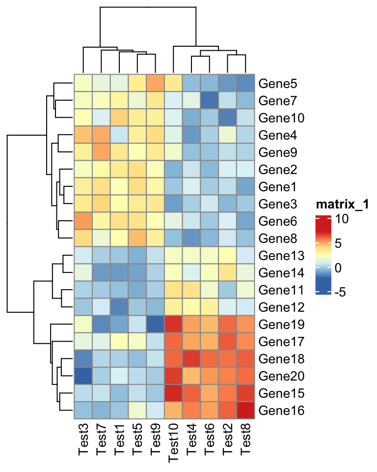
Everything looks the same except the style of the heatmap legend. There are also some other visual difference which you can find in the “Comparisons” section in this post.
The next one is an example for setting annotations (you should be familiar with how to set these data frames and color list if you are a pheatmap user).
annotation_col = data.frame(
    CellType = factor(rep(c("CT1", "CT2"), 5)),
    Time = 1:5
)
rownames(annotation_col) = paste("Test", 1:10, sep = "")

annotation_row = data.frame(
    GeneClass = factor(rep(c("Path1", "Path2", "Path3"), c(10, 4, 6)))
)
rownames(annotation_row) = paste("Gene", 1:20, sep = "")

ann_colors = list(
    Time = c("white", "firebrick"),
    CellType = c(CT1 = "#1B9E77", CT2 = "#D95F02"),
    GeneClass = c(Path1 = "#7570B3", Path2 = "#E7298A", Path3 = "#66A61E")
)
pheatmap(test, annotation_col = annotation_col, annotation_row = annotation_row,
    annotation_colors = ann_colors)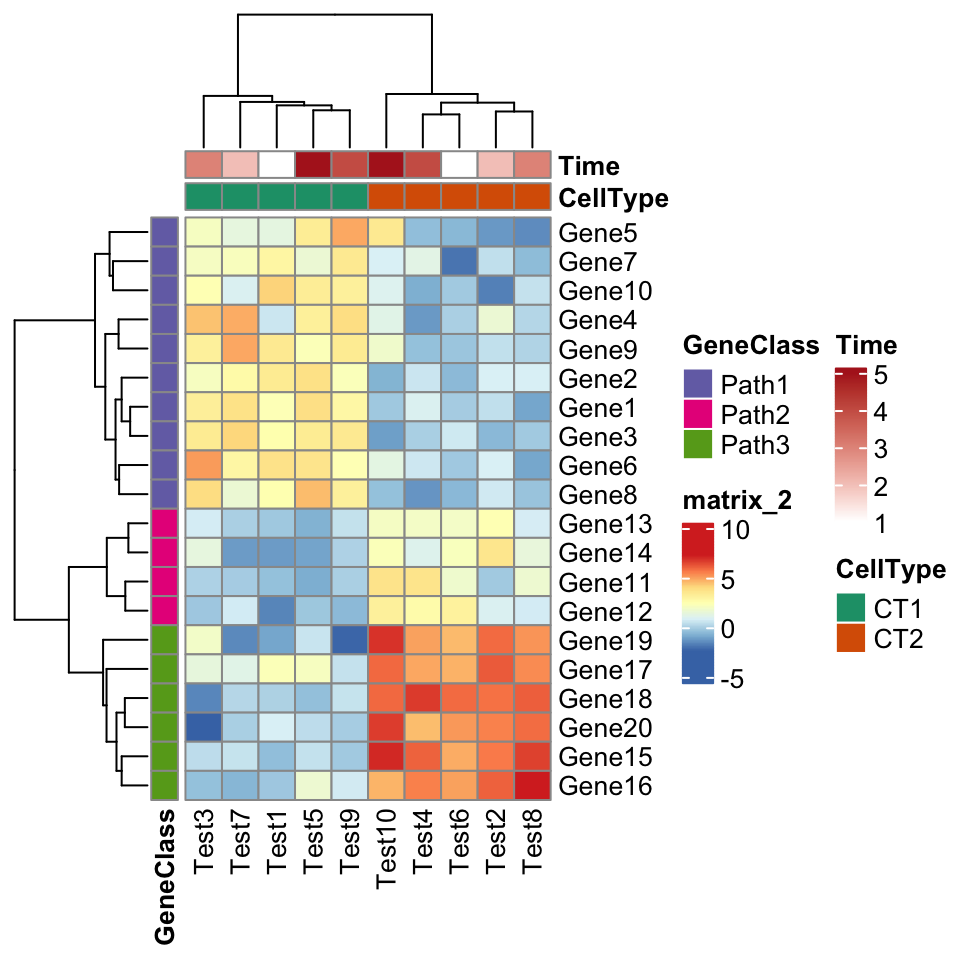
ComplexHeatmap::pheatmap() returns a Heatmap object, so it can be added with
other heatmaps and annotations. Or in other words, you can add multiple pheatmaps
and annotations. Cool!
p1 = pheatmap(test, name = "mat1")
p2 = rowAnnotation(foo = anno_barplot(1:nrow(test)))
p3 = pheatmap(test, name = "mat2",
    col = colorRampPalette(c("navy", "white", "firebrick3"))(50))
# or you can simply specify as
# p3 = pheatmap(test, name = "mat2", col = c("navy", "white", "firebrick3"))
p1 + p2 + p3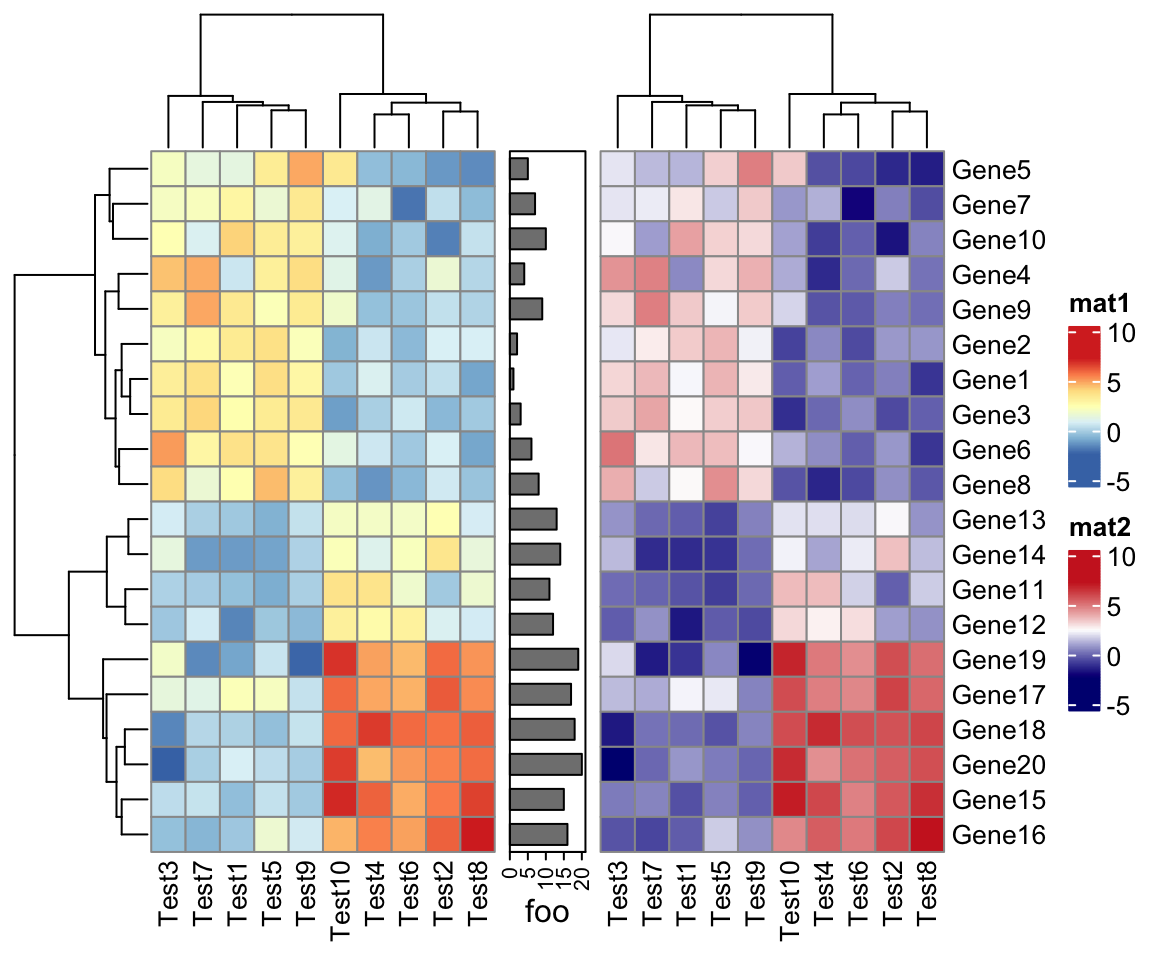
Nevertheless, if you really want to add multiple pheatmaps, I still suggest you
to directly use the Heatmap() function. You can find how to migrate from
pheatmap::pheatmap() to ComplexHeatmap::Heatmap() in the next section.
In previous examples, the legend for row annotation is grouped with heatmap legend.
This can be modified by setting legend_grouping argument in draw() function:
p = pheatmap(test, annotation_col = annotation_col, annotation_row = annotation_row,
    annotation_colors = ann_colors)
draw(p, legend_grouping = "original")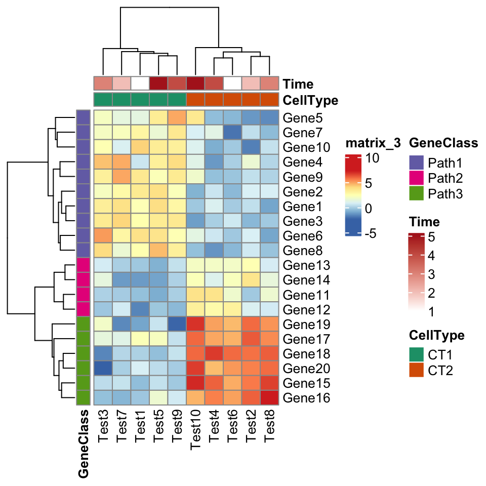
One last thing is since ComplexHeatmap::pheatmap() returns a Heatmap object,
if pheatmap() is not called in an interactive environment, e.g. in an R script,
inside a function or in a for loop, you need to explicitly use draw() function:
for(...) {
    p = pheatmap(...)
    draw(p)
}
10.1.2 Translation
Following table lists how to map parameters in pheatmap::pheatmap() to ComplexHeatmap::Heatmap().
Arguments in pheatmap::pheatmap()
|
Identical settings/arguments in ComplexHeatmap::Heatmap()
|
|---|---|
mat |
matrix |
color |
Users can specify a color mapping function by circlize::colorRamp2(), or provide a vector of colors on which colors for individual values are linearly interpolated. |
kmeans_k |
No corresponding parameter because it changes the matrix for heatmap. |
breaks |
It should be specified in the color mapping function. |
border_color |
rect_gp = gpar(col = border_color). In the annotations, it is HeatmapAnnotation(..., gp = gpar(col = border_color)). |
cellwidth |
width = ncol(mat)*unit(cellwidth, "pt") |
cellheight |
height = nrow(mat)*unit(cellheight, "pt") |
scale |
Users should simply apply scale() on the matrix before sending to Heatmap(). |
cluster_rows |
cluster_rows |
cluster_cols |
cluster_columns |
clustering_distance_rows |
clustering_distance_rows. The value correlation should be changed to pearson. |
clustering_distance_cols |
clustering_distance_columns, The value correlation should be changed to pearson. |
clustering_method |
clustering_method_rows/clustering_method_columns
|
clustering_callback |
The processing on the dendrogram should be applied before sending to Heatmap(). |
cutree_rows |
row_split and row clustering should be applied. |
cutree_cols |
column_split and column clustering should be applied. |
treeheight_row |
row_dend_width = unit(treeheight_row, "pt") |
treeheight_col |
column_dend_height = unit(treeheight_col, "pt") |
legend |
show_heatmap_legend |
legend_breaks |
heatmap_legend_param = list(at = legend_breaks) |
legend_labels |
heatmap_legend_param = list(labels = legend_labels) |
annotation_row |
left_annotatioin = rowAnnotation(df = annotation_row) |
annotation_col |
top_annotation = HeatmapAnnotation(df = annotation_col) |
annotation |
Not supported. |
annotation_colors |
col argument in HeatmapAnnotation()/rowAnnotation(). |
annotation_legend |
show_legend argument in HeatmapAnnotation()/rowAnnotation(). |
annotation_names_row |
show_annotation_name in rowAnnotation(). |
annotation_names_col |
show_annotation_name in HeatmaoAnnotation(). |
drop_levels |
Unused levels are all dropped. |
show_rownames |
show_row_names |
show_colnames |
show_column_names |
main |
column_title |
fontsize |
gpar(fontsize = fontsize) in corresponding heatmap components. |
fontsize_row |
row_names_gp = gpar(fontsize = fontsize_row) |
fontsize_col |
column_names_gp = gpar(fontsize = fontsize_col) |
angle_col |
column_names_rot. The rotation of row annotation names are not supported. |
display_numbers |
Users should set a proper cell_fun or layer_fun (vectorized and faster version of cell_fun). E.g. if display_numbers is TRUE, layer_fun can be set as function(j, i, x, y, w, h, fill) { grid.text(sprintf(number_format, pindex(mat, i, j)), x = x, y = y, gp = gpar(col = number_color, fontsize = fontsize_number)) }. If display_numbers is a matrix, replace mat to display_numbers in the layer_fun. |
number_format |
See above. |
number_color |
See above. |
fontsize_number |
See above. |
gaps_row |
Users should construct a “splitting variable” and send to row_split. E.g. slices = diff(c(0, gaps_row, nrow(mat))); rep(seq_along(slices), times = slices). |
gaps_col |
Users should construct a “splitting variable” and send to column_split. |
labels_row |
row_labels |
labels_col |
column_labels |
filename |
No corresponding setting in Heatmap(). Users need to explicitly use e.g. pdf(). |
width |
No corresponding setting in Heatmap(). |
height |
No corresponding setting in Heatmap(). |
silent |
No corresponding setting in Heatmap(). |
na_col |
na_col |
10.1.3 Comparisons
I ran all the example code in the “Examples” section of the documentation of
pheatmap::pheatmap() function .
I also implemented a wrapper function ComplexHeatmap::compare_pheatmap() which basically uses the same
set of arguments for pheatmap::pheatmap() and ComplexHeatmap::pheatmap() and
draws two heatmaps, so that you can directly see the similarity and difference
of the two heatmap implementations.
compare_pheatmap(test)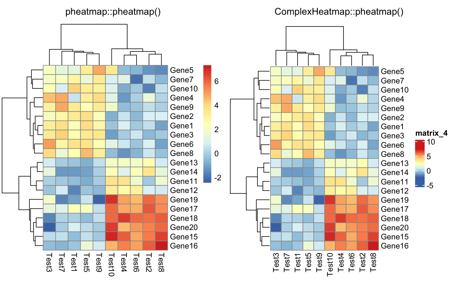
compare_pheatmap(test, scale = "row", clustering_distance_rows = "correlation")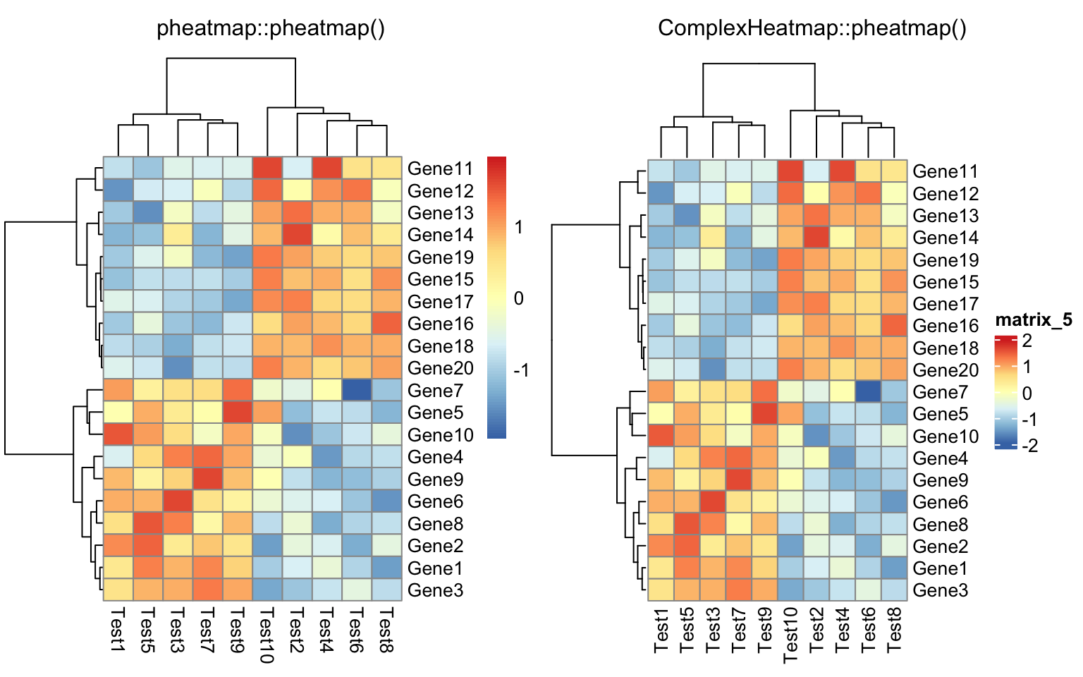
compare_pheatmap(test,
    color = colorRampPalette(c("navy", "white", "firebrick3"))(50))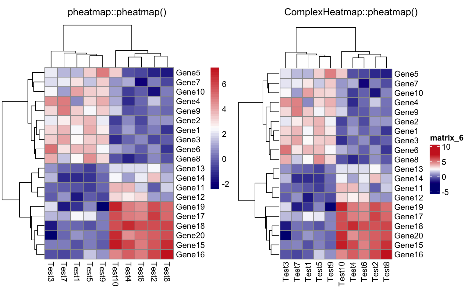
compare_pheatmap(test, cluster_row = FALSE)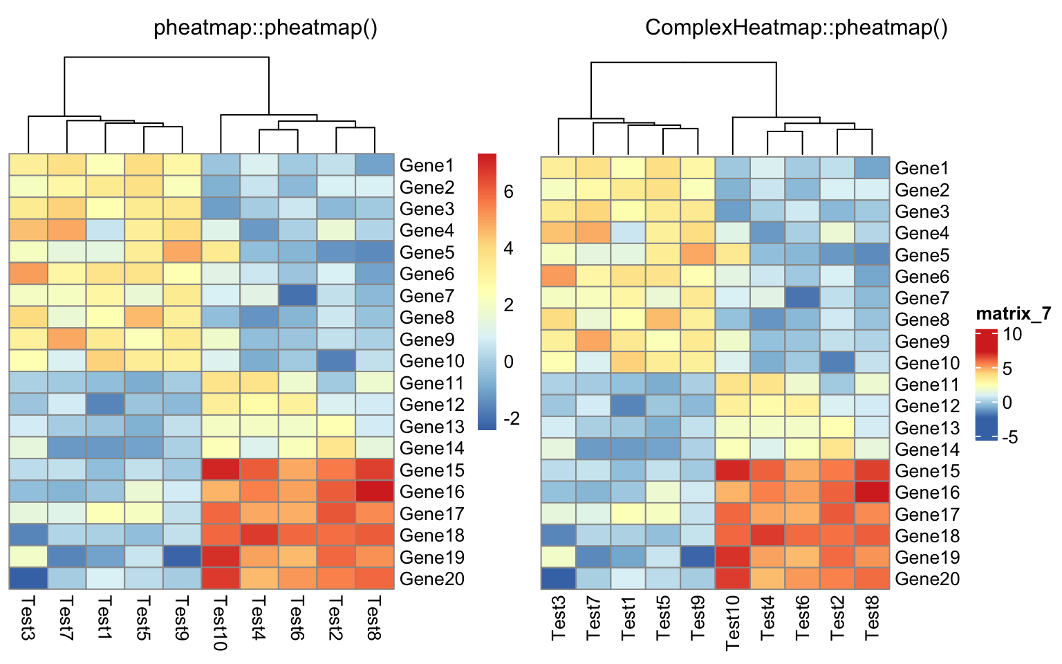
compare_pheatmap(test, legend = FALSE)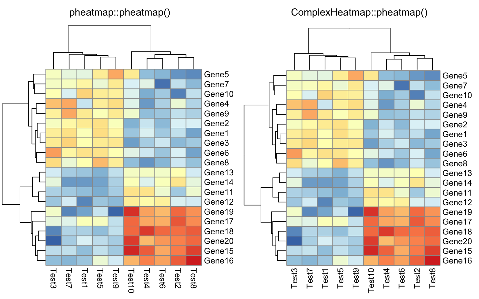
compare_pheatmap(test, display_numbers = TRUE)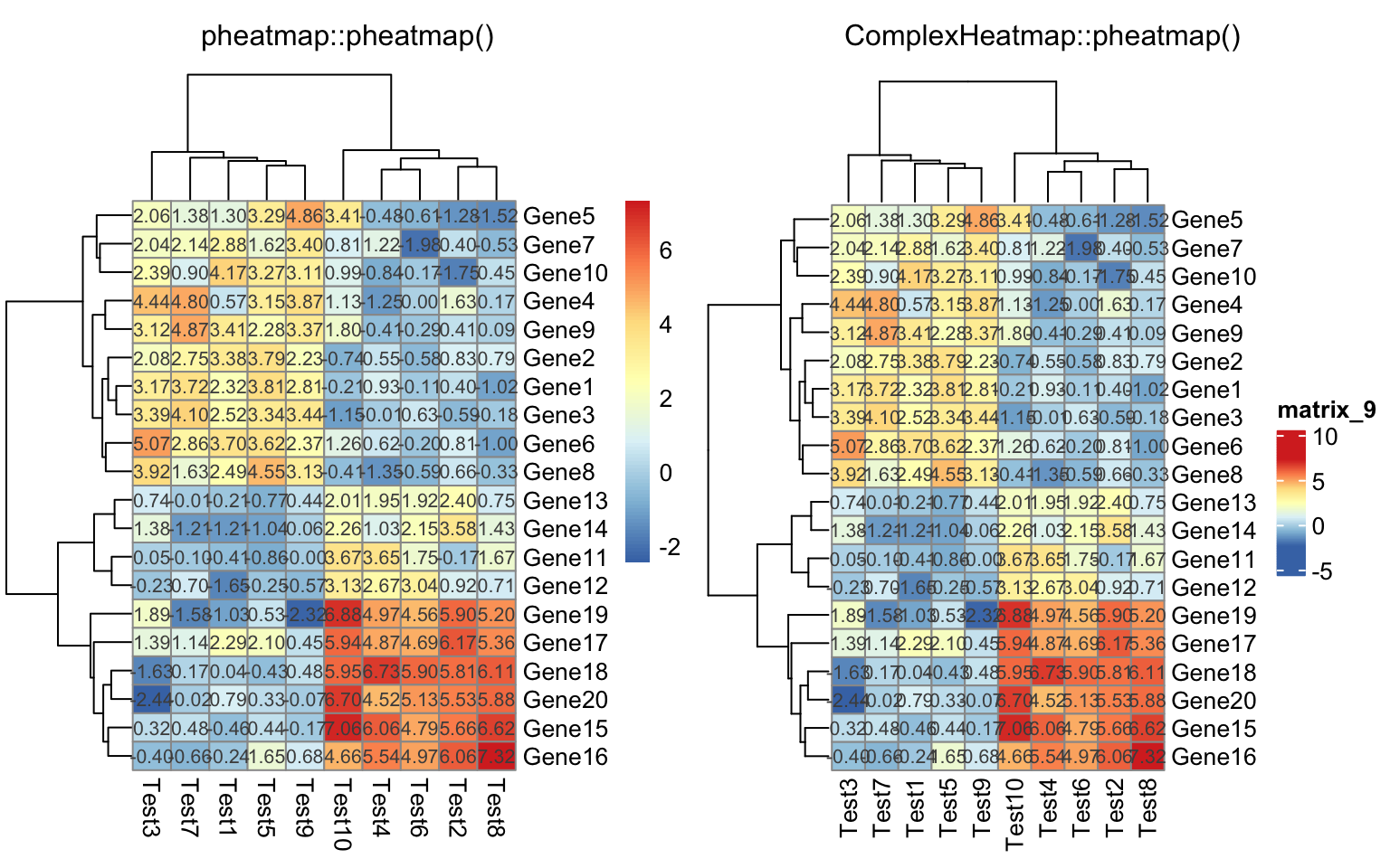
compare_pheatmap(test, display_numbers = TRUE, number_format = "%.1e")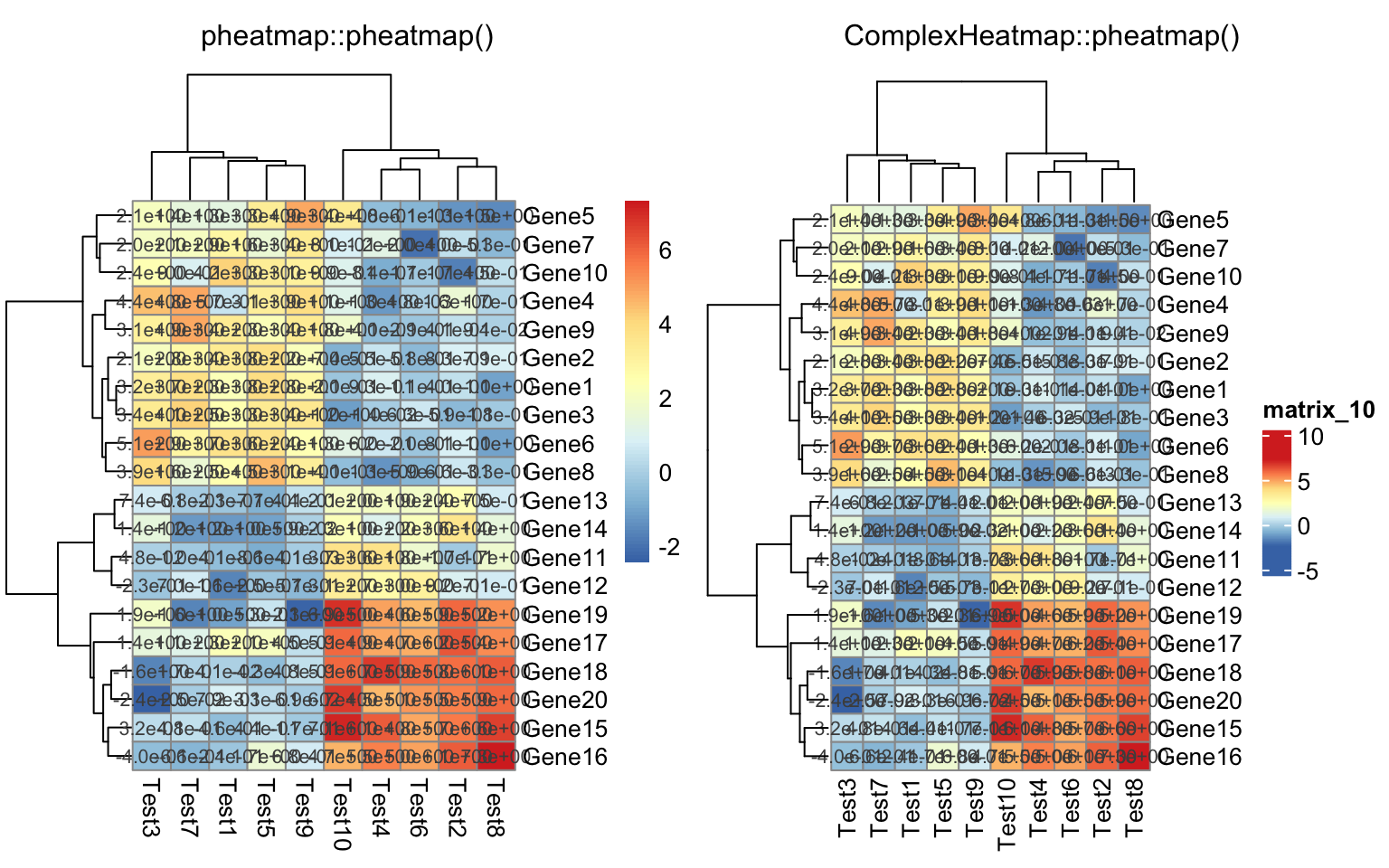
compare_pheatmap(test,
    display_numbers = matrix(ifelse(test > 5, "*", ""), nrow(test)))
compare_pheatmap(test, cluster_row = FALSE, legend_breaks = -1:4,
    legend_labels = c("0", "1e-4", "1e-3", "1e-2", "1e-1", "1"))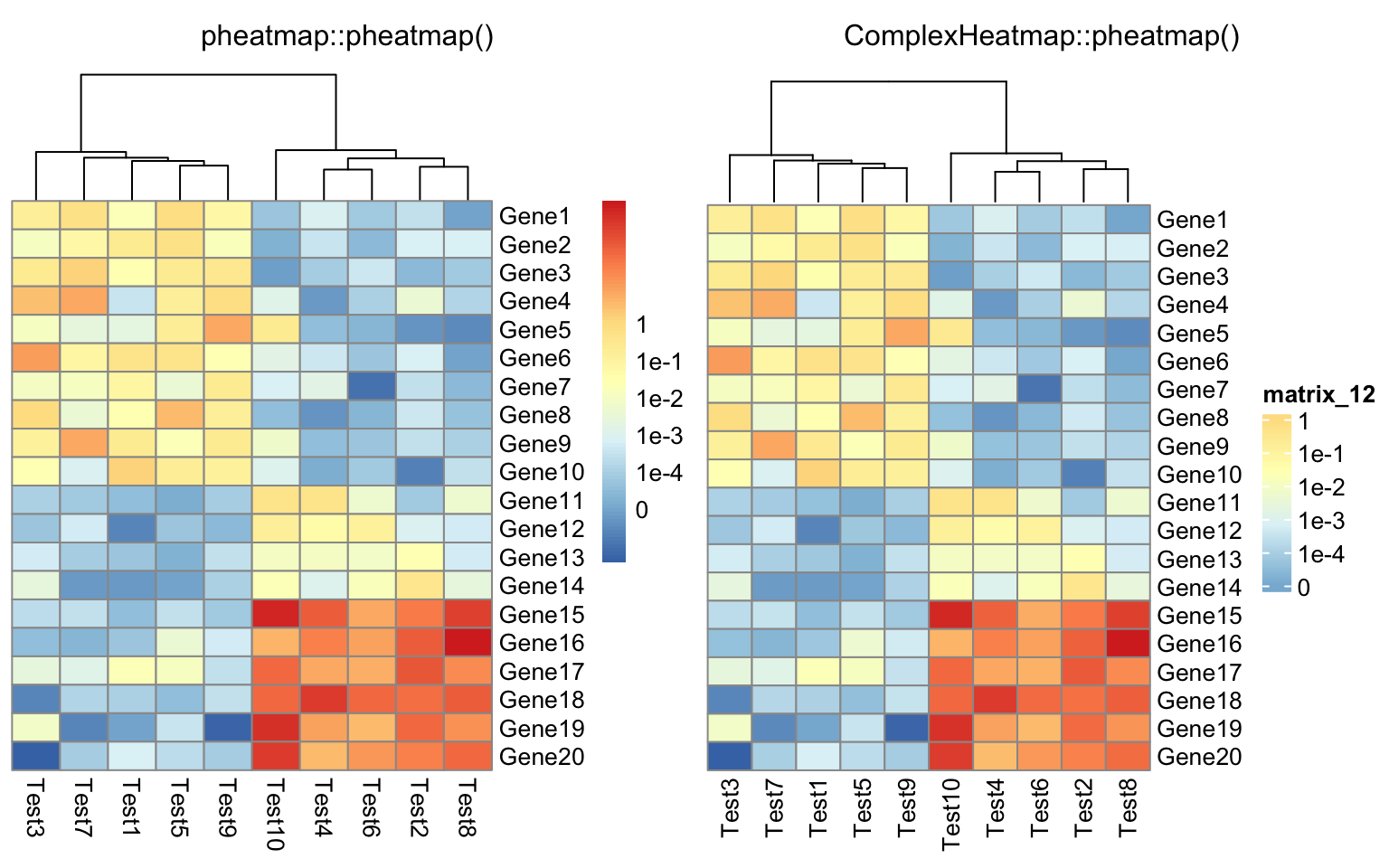
compare_pheatmap(test, cellwidth = 15, cellheight = 12, main = "Example heatmap")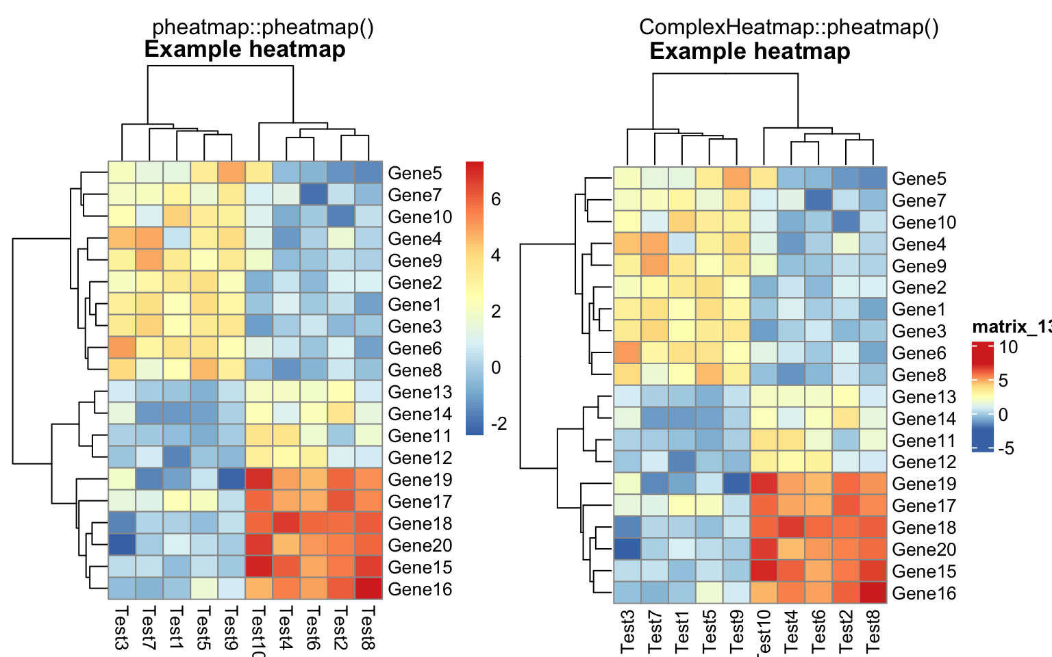
annotation_col = data.frame(
    CellType = factor(rep(c("CT1", "CT2"), 5)),
    Time = 1:5
)
rownames(annotation_col) = paste("Test", 1:10, sep = "")

annotation_row = data.frame(
    GeneClass = factor(rep(c("Path1", "Path2", "Path3"), c(10, 4, 6)))
)
rownames(annotation_row) = paste("Gene", 1:20, sep = "")

compare_pheatmap(test, annotation_col = annotation_col)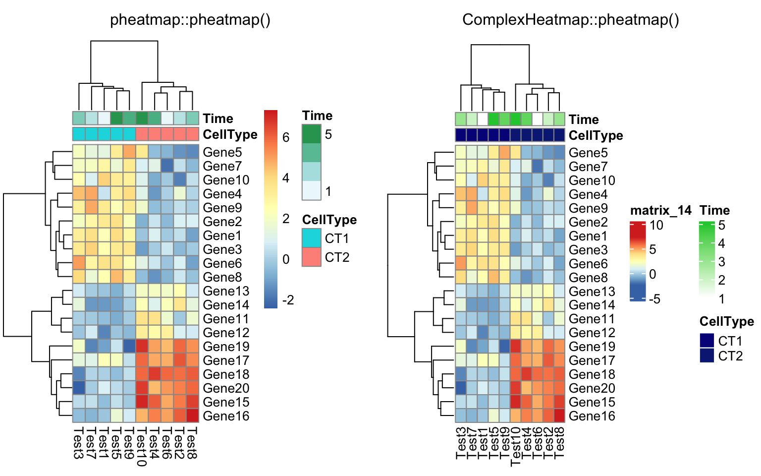
compare_pheatmap(test, annotation_col = annotation_col, annotation_legend = FALSE)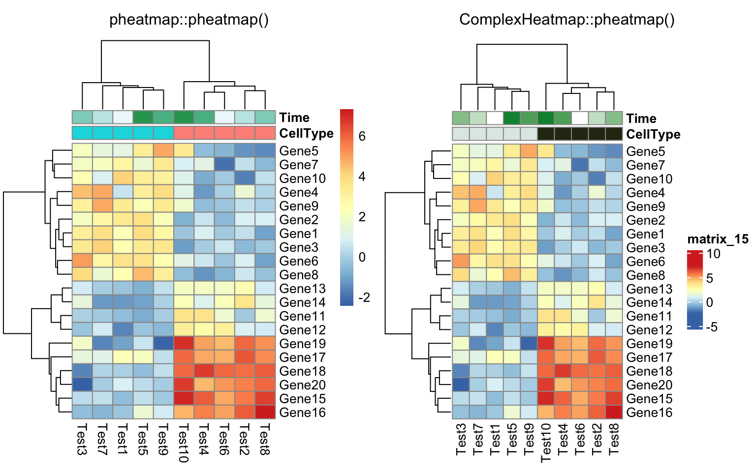
compare_pheatmap(test, annotation_col = annotation_col,
    annotation_row = annotation_row)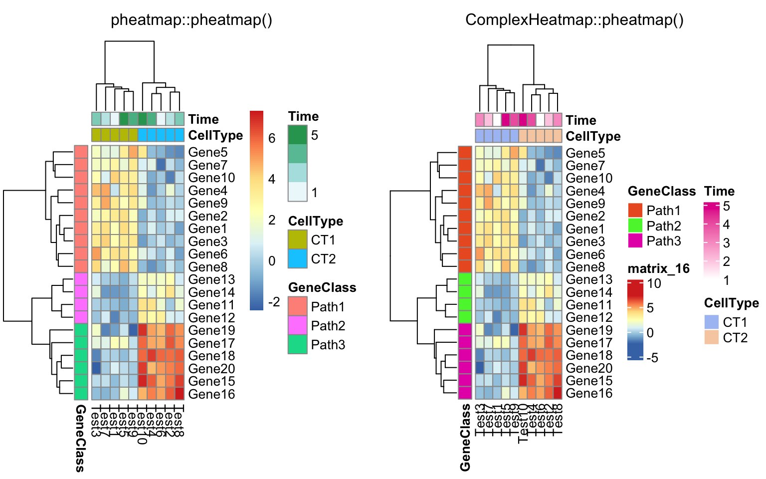
compare_pheatmap(test, annotation_col = annotation_col,
    annotation_row = annotation_row, angle_col = "45")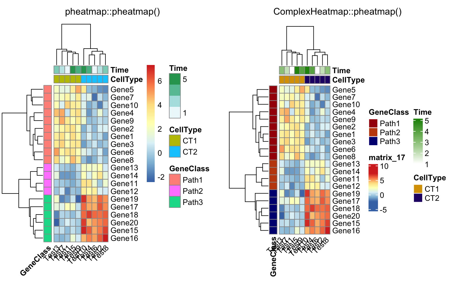
compare_pheatmap(test, annotation_col = annotation_col, angle_col = "0")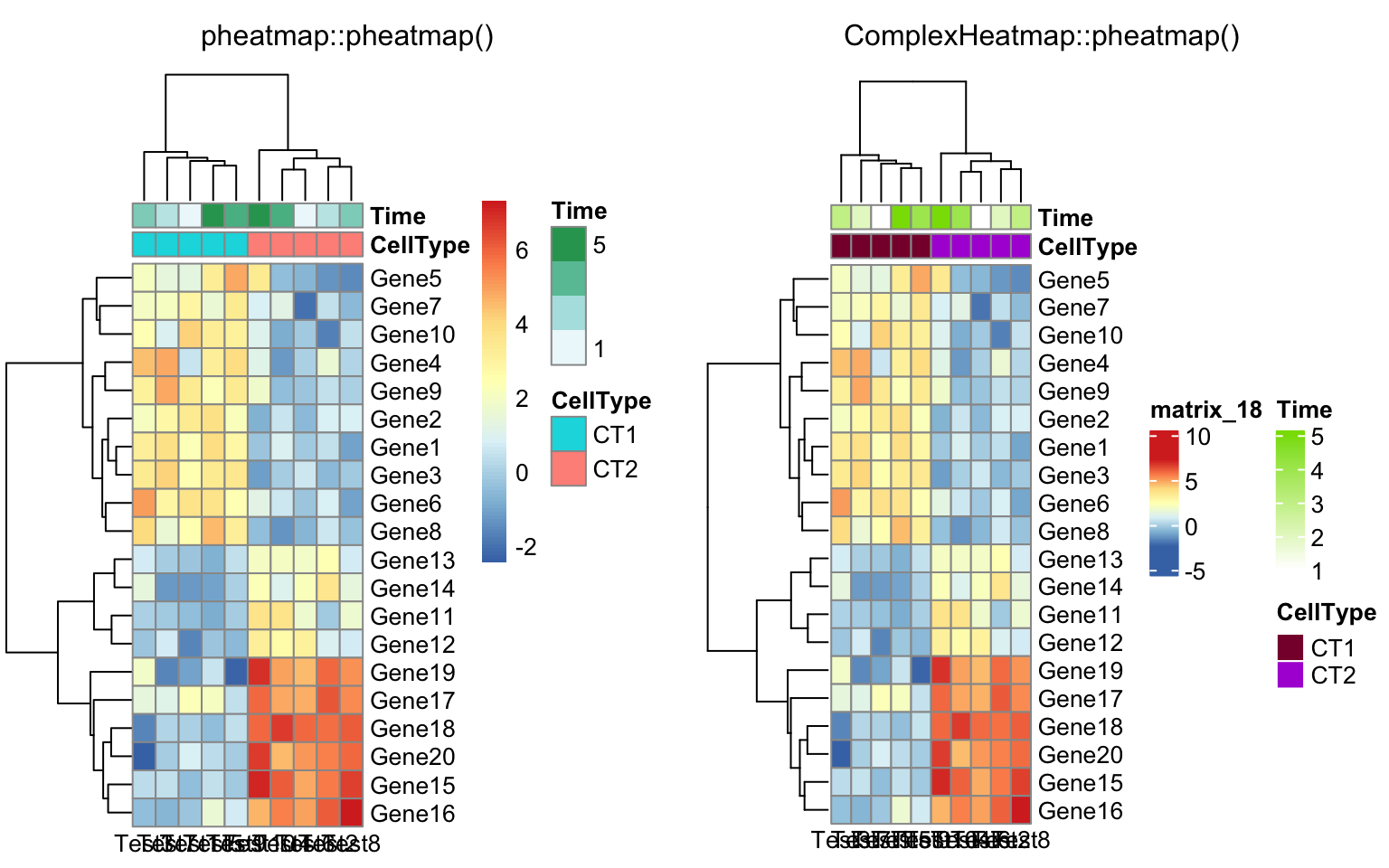
ann_colors = list(
    Time = c("white", "firebrick"),
    CellType = c(CT1 = "#1B9E77", CT2 = "#D95F02"),
    GeneClass = c(Path1 = "#7570B3", Path2 = "#E7298A", Path3 = "#66A61E")
)

compare_pheatmap(test, annotation_col = annotation_col,
    annotation_colors = ann_colors, main = "Title")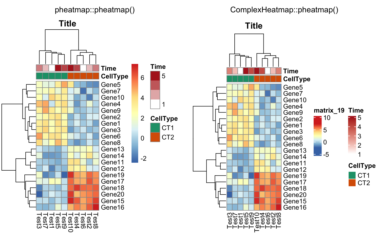
compare_pheatmap(test, annotation_col = annotation_col,
    annotation_row = annotation_row, annotation_colors = ann_colors)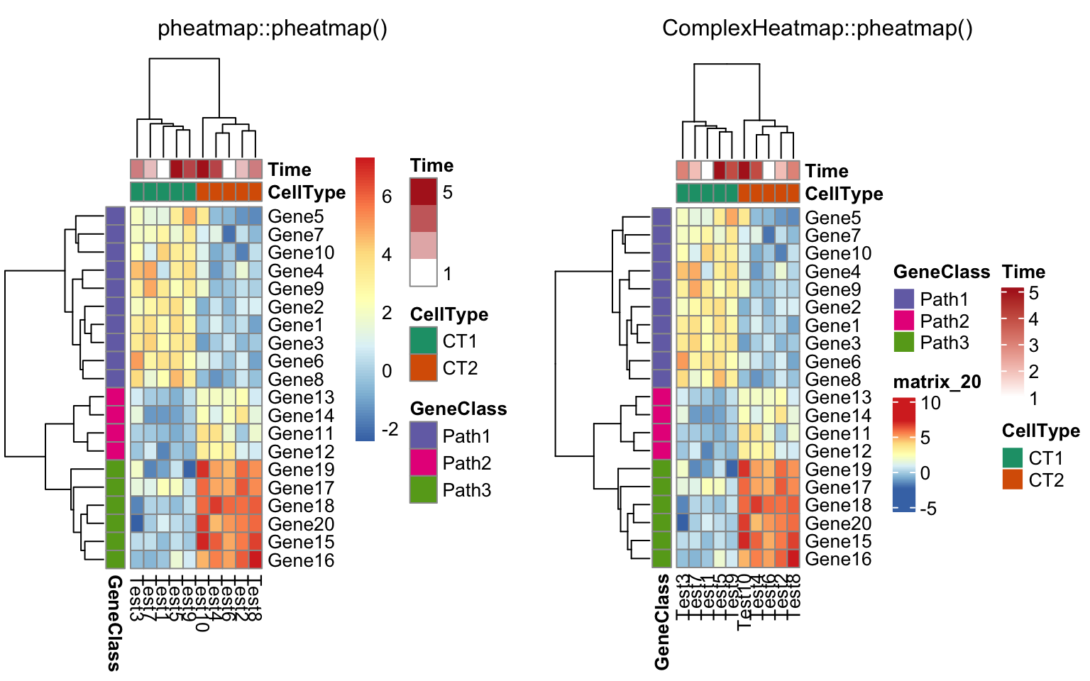
compare_pheatmap(test, annotation_col = annotation_col,
annotation_colors = ann_colors[2]) 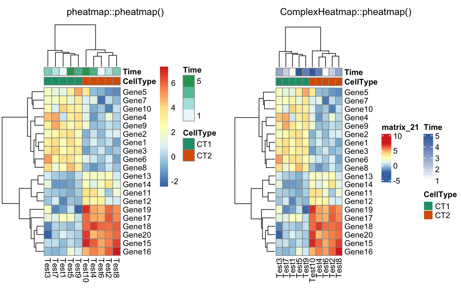
compare_pheatmap(test, annotation_col = annotation_col, cluster_rows = FALSE,
    gaps_row = c(10, 14))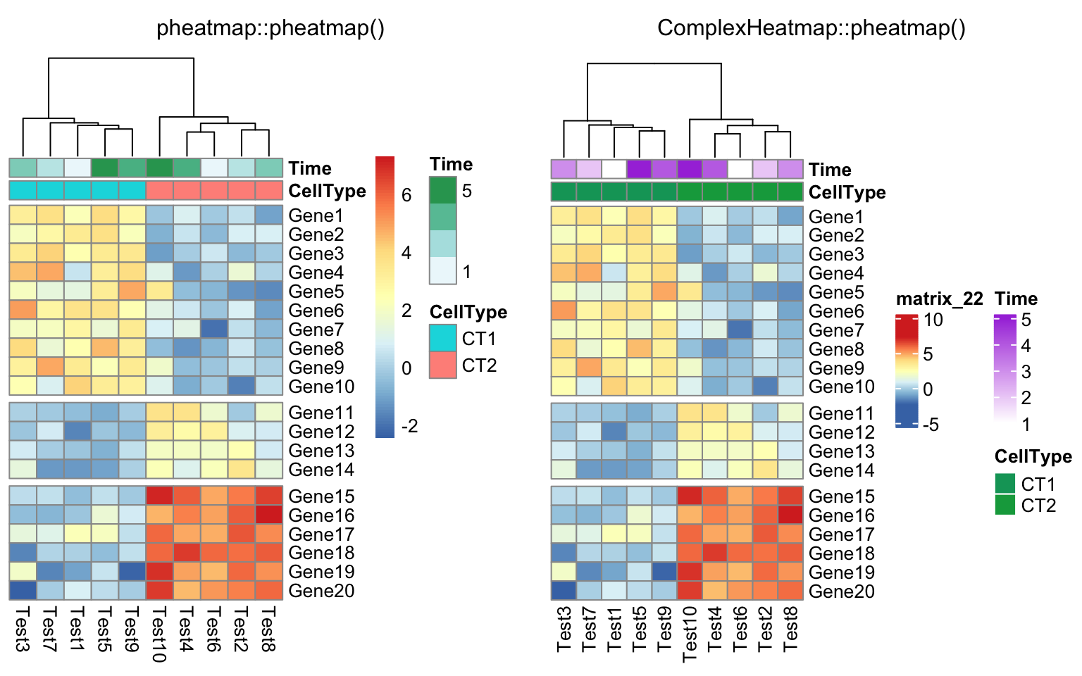
compare_pheatmap(test, annotation_col = annotation_col, cluster_rows = FALSE,
    gaps_row = c(10, 14), cutree_col = 2)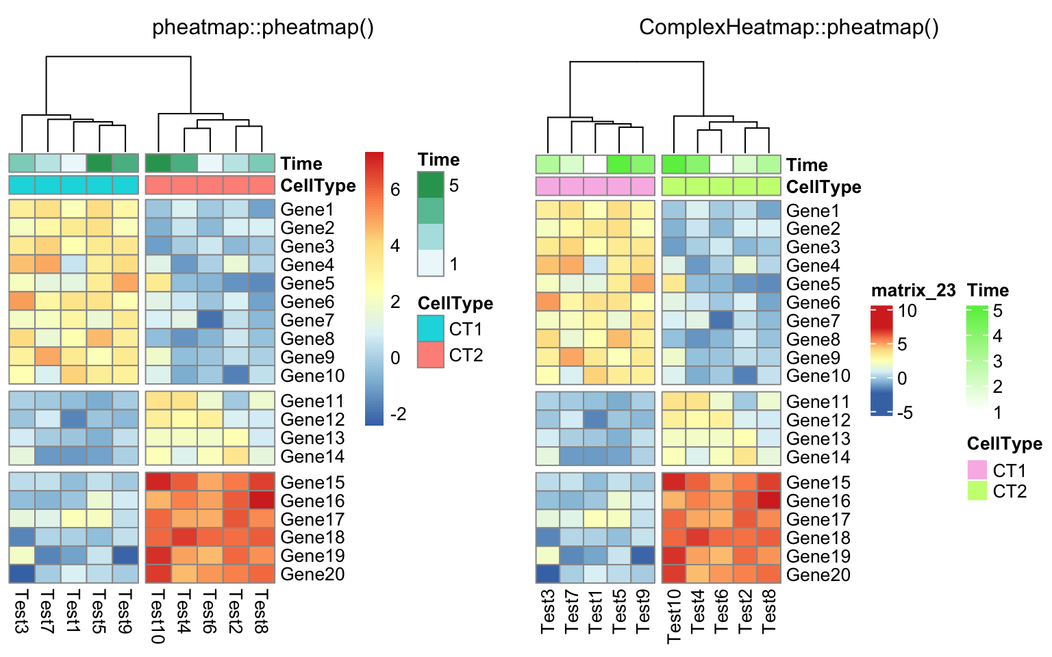
labels_row = c("", "", "", "", "", "", "", "", "", "", "", "", "", "", "",
    "", "", "Il10", "Il15", "Il1b")
compare_pheatmap(test, annotation_col = annotation_col, labels_row = labels_row)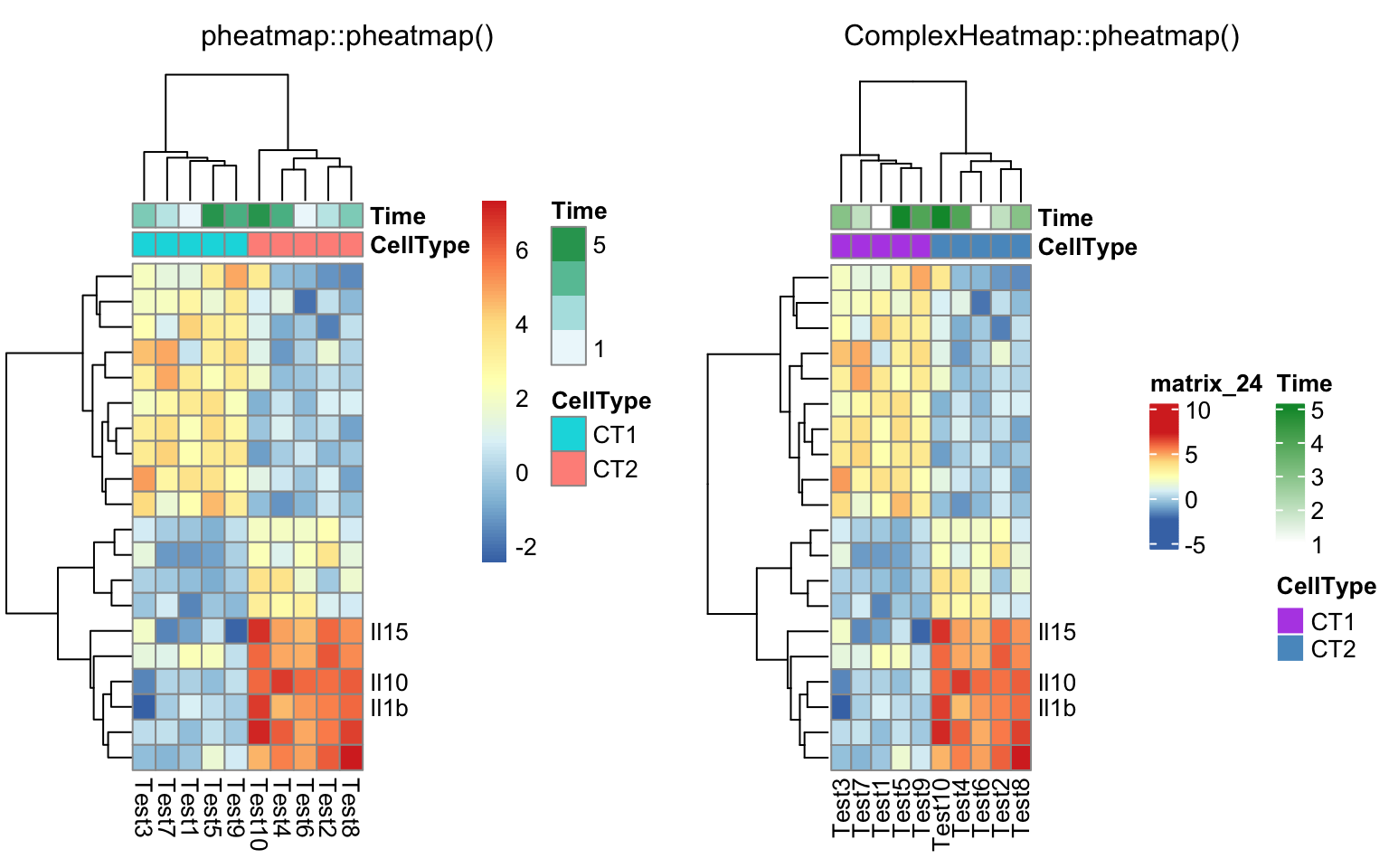
drows = dist(test, method = "minkowski")
dcols = dist(t(test), method = "minkowski")
compare_pheatmap(test, clustering_distance_rows = drows,
    clustering_distance_cols = dcols)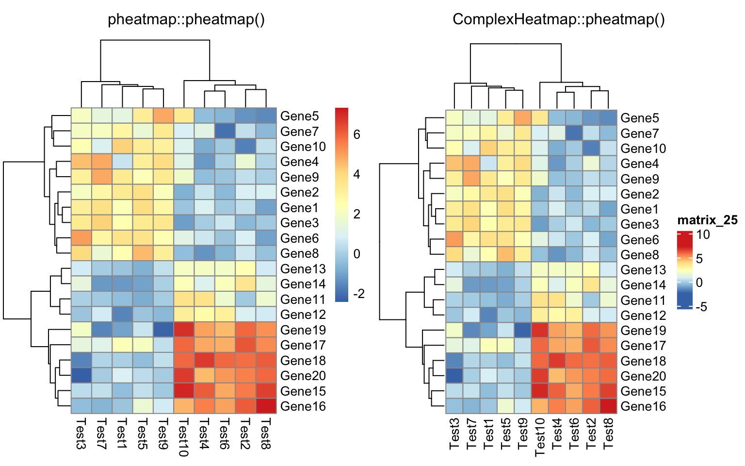
library(dendsort)
callback = function(hc, ...){dendsort(hc)}
compare_pheatmap(test, clustering_callback = callback)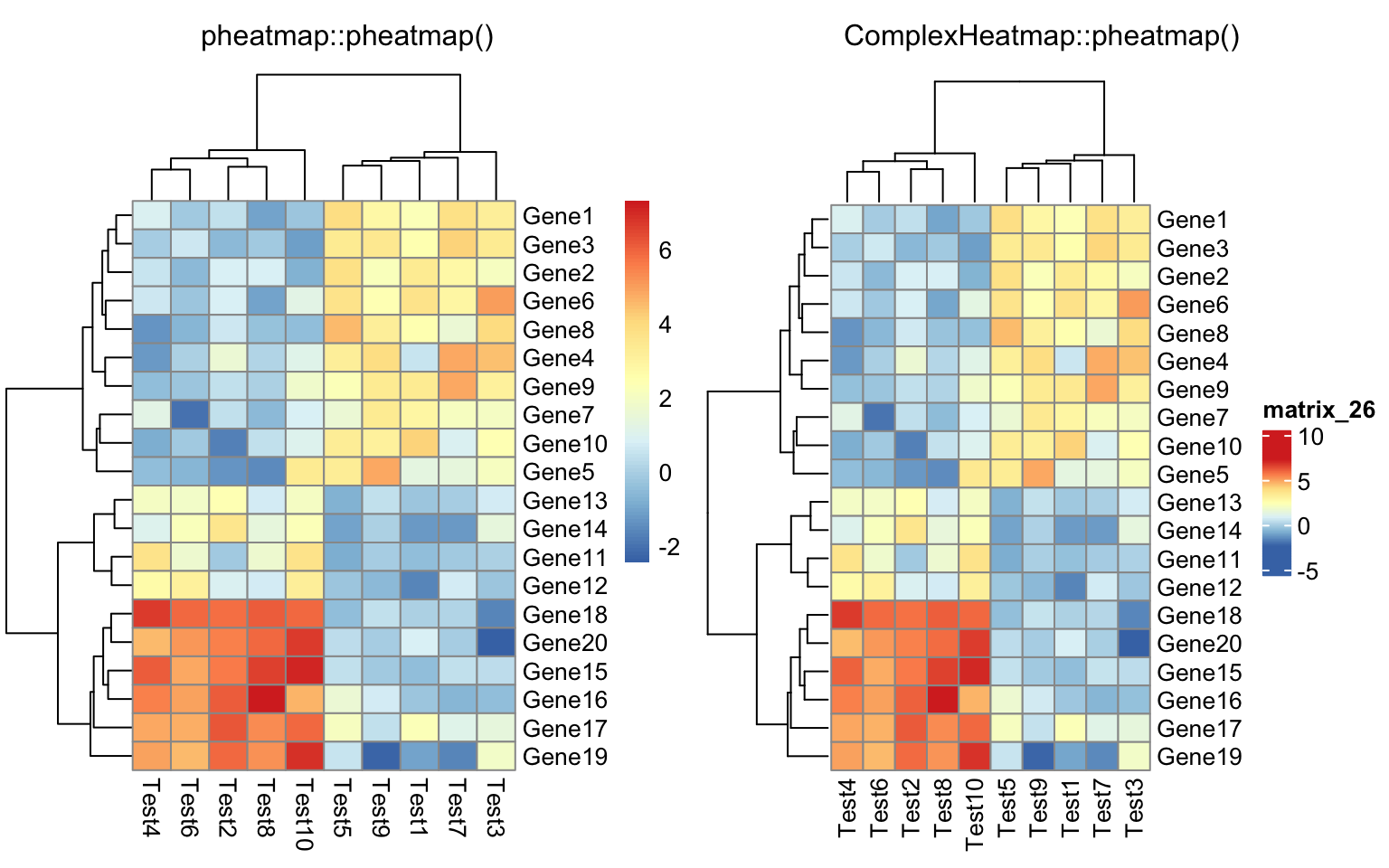
10.2 cowplot
The cowplot package is used to combine multiple plots into a single figure. In most cases, ComplexHeatmap works perfectly with cowplot, but there are some cases that need special attention.
Also there are some other packages that combine multiple plots, such as multipanelfigure, but I think the mechanism behind is the same.
Following functionalities in ComplexHeatmap cause problems with using cowplot.
-
anno_zoom()/anno_link(): The adjusted positions by these two functions rely on the size of the graphics device. -
anno_mark(): The same reason asanno_zoom(). The adjusted positions also rely on the device size. - When there are too many legends, the legends will be wrapped into multiple columns. The calculation of the legend positions rely on the device size.
In following I demonstrate a case with using the anno_zoom(). Here the
example is from the simplifyEnrichment
package and the plot shows a
GO similarity heatmap with word cloud annotation showing the major biological
functions in each group.
You don’t need to really understand the following code. The ht_clusters()
function basically draws a heatmap with Heatmap() and add the word cloud
annotation by anno_zoom().
library(simplifyEnrichment)
set.seed(1234)
go_id = random_GO(500)
mat = GO_similarity(go_id)
cl = binary_cut(mat)
ht_clusters(mat, cl)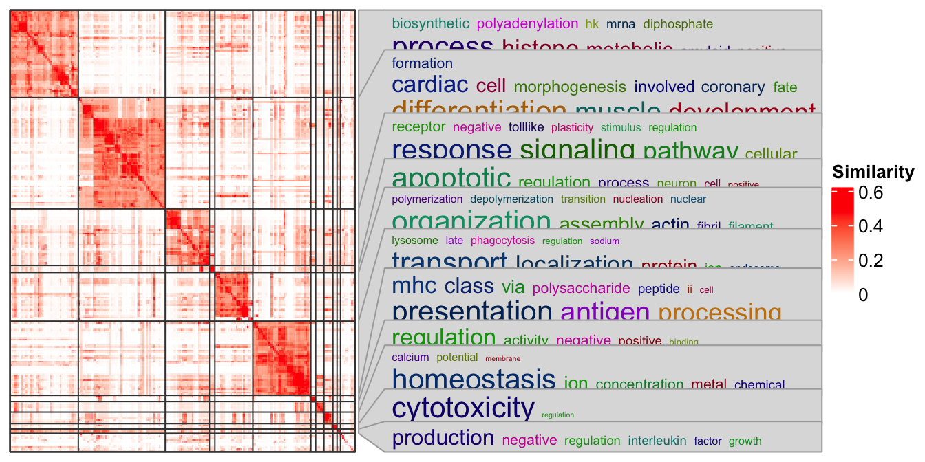
Next we put this heatmap as a sub-figure with cowplot. To integrate with
cowplot, the heatmap should be captured by grid::grid.grabExpr() as a complex
grob object. Note here you need to use draw() function to draw the heatmap
explicitly.
library(cowplot)
library(grid)
p1 = rectGrob(width = 0.9, height = 0.9)
p2 = grid.grabExpr(ht_clusters(mat, cl))
p3 = rectGrob(width = 0.9, height = 0.9)

plot_grid(p1,
    plot_grid(p2, p3, nrow = 2, rel_heights = c(4, 1)),
    nrow = 1, rel_widths = c(1, 9)
)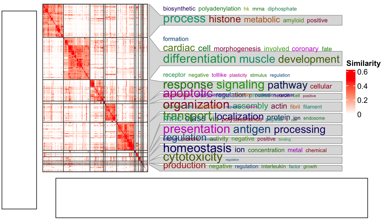
Woooo! The word cloud annotation is badly aligned.
There are some details that should be noted for grid.grabExpr() function. It actually
opens an invisible graphics device (by pdf(NULL)) with a default size 7x7 inches. Thus,
for this line:
p2 = grid.grabExpr(ht_clusters(mat, cl))The word cloud annotation in p2 is actually calculated in a region of 7x7
inches, and when it is written back to the figure by plot_grid(), the space
for p2 changes, that is why the word cloud annotation is wrongly aligned.
On the other hand, if “a simple heatmap” is captured by grid.grabExpr(), e.g.:
p2 = grid.grabExpr(draw(Heatmap(mat)))when p2 is put back, everything will work fine because now all the heatmap
elements are not dependent on the device size and the positions will be
automatically adjusted to the new space.
This effect can also be observed by plotting the heatmap in the interactive graphics device and resizing the window by dragging it.
The solution is rather simple. Since the reason for this inconsistency is the different space between where it is captured and where it is drawn, we only need to capture the heatmap under the device with the same size as where it is going to be put.
As in the layout which we set in the plot_grid() function, the heatmap occupies
9/10 width and 4/5 height of the figure. So, the width and height of the space
for the heatmap is calculated as follows and assigned to the width and
height arguments in grid.grabExpr().
w = convertWidth(unit(1, "npc")*(9/10), "inch", valueOnly = TRUE)
h = convertHeight(unit(1, "npc")*(4/5), "inch", valueOnly = TRUE)
p2 = grid.grabExpr(ht_clusters(mat, cl), width = w, height = h)

plot_grid(p1,
    plot_grid(p2, p3, nrow = 2, rel_heights = c(4, 1)),
    nrow = 1, rel_widths = c(1, 9)
)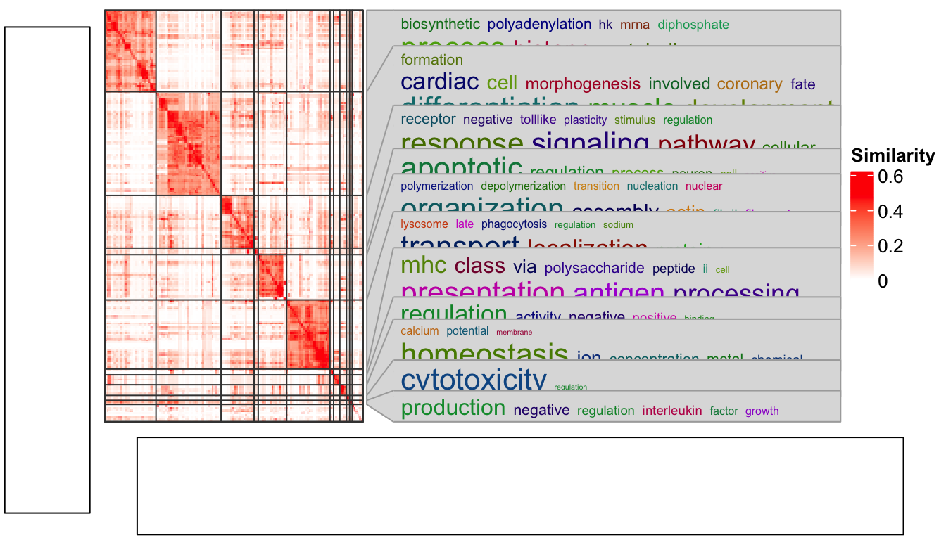
Now everthing is back to normal!
10.3 gridtext
The gridtext package provides a nice and easy way for rendering text under the grid system. From version 2.3.3 of ComplexHeatmap, text-related elements can be rendered by gridtext.
For all text-related elements, the text needs to be wrapped by gt_render() function, which marks
the text and adds related parameters that are going to be processed by gridtext.
Currently ComplexHeatmap supports gridtext::richtext_grob(), so some of the parameters for
richtext_grob() can be passed via gt_render().
## [1] "foo"
## attr(,"class")
## [1] "gridtext"
## attr(,"param")
## attr(,"param")$r
## [1] 2points
##
## attr(,"param")$padding
## [1] 2points 2points 2points 2points
For each heatmap element, e.g. column title, graphic parameters can be set by the companion argument,
e.g. column_title_gp. To make it simpler, all graphic parameters set by box_gp are merged with *_gp
by adding box_ prefix, e.g.:
..., column_title = gt_render("foo"), column_title_gp = gpar(col = "red", box_fill = "blue"), ...Graphic parameters can also be specified inside gt_render(). Following is the same as the one above:
..., column_title = gt_render("foo", gp = gpar(col = "red", box_fill = "blue")), ...10.3.1 Titles
set.seed(123)
mat = matrix(rnorm(100), 10)
rownames(mat) = letters[1:10]
Heatmap(mat,
    column_title = gt_render("Some <span style='color:blue'>blue text **in bold.**</span><br>And *italics text.*<br>And some <span style='font-size:18pt; color:black'>large</span> text.",
        r = unit(2, "pt"),
        padding = unit(c(2, 2, 2, 2), "pt")),
    column_title_gp = gpar(box_fill = "orange"))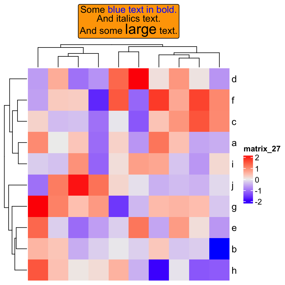
If heatmap is split:
Heatmap(mat,
    row_km = 2,
    row_title = gt_render(c("**title1**", "_title2_")),
    row_title_gp = gpar(box_fill = c("yellow", "blue")))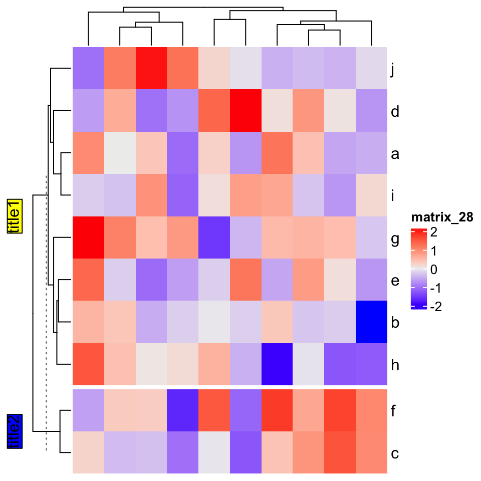
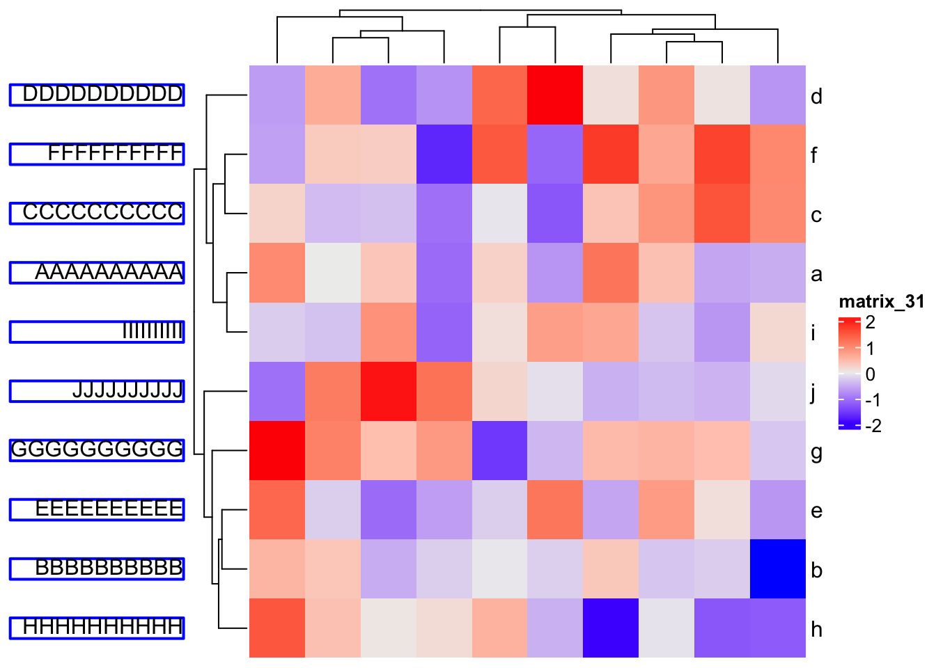
10.3.2 Row/column names
Rendered row/column names should be explicitly specified by row_labels/column_labels
Heatmap(mat,
    row_labels = gt_render(letters[1:10], padding = unit(c(2, 10, 2, 10), "pt")),
    row_names_gp = gpar(box_col = rep(c("red", "green"), times = 5)))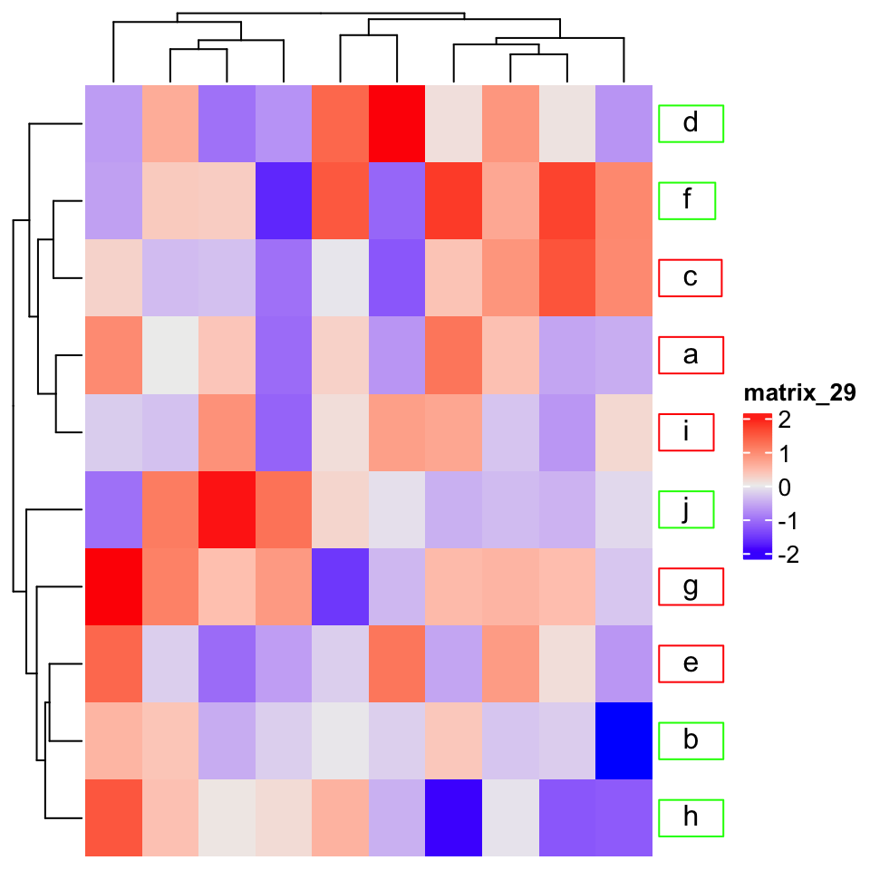
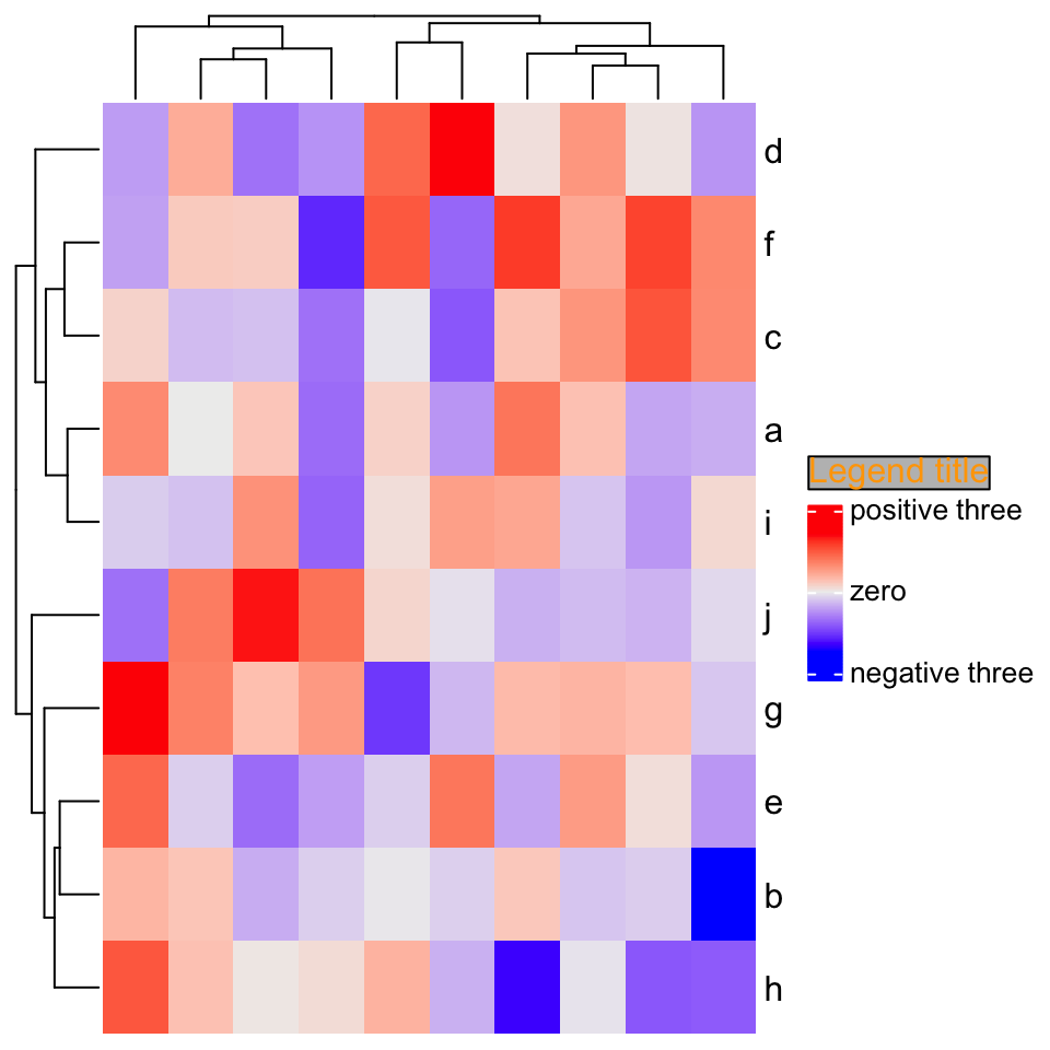
10.3.3 Annotation labels
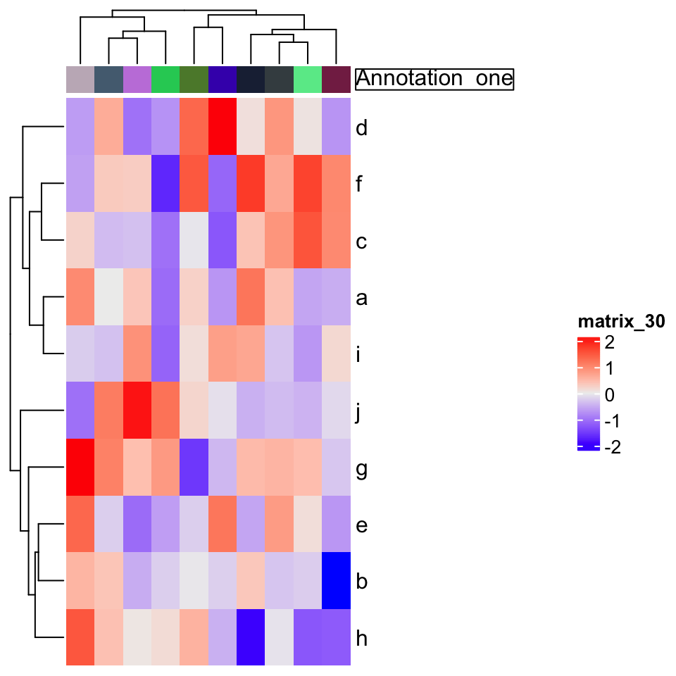
annotation_label argument should be as rendered text.
ha = HeatmapAnnotation(foo = letters[1:10],
    annotation_label = gt_render("**Annotation** _one_",
        gp = gpar(box_col = "black")),
    show_legend = FALSE)
Heatmap(mat, top_annotation = ha)