2 A Single Heatmap
A single heatmap is the most used approach for visualizing data. Although “the shining point” of the ComplexHeatmap package is that it can visualize a list of heatmaps in parallel, however, as the basic unit of the heatmap list, it is still very important to have the single heatmap well configured.
First let’s generate a random matrix where there are three groups in the columns and three groups in the rows:
set.seed(123)
nr1 = 4; nr2 = 8; nr3 = 6; nr = nr1 + nr2 + nr3
nc1 = 6; nc2 = 8; nc3 = 10; nc = nc1 + nc2 + nc3
mat = cbind(rbind(matrix(rnorm(nr1*nc1, mean = 1,   sd = 0.5), nr = nr1),
          matrix(rnorm(nr2*nc1, mean = 0,   sd = 0.5), nr = nr2),
          matrix(rnorm(nr3*nc1, mean = 0,   sd = 0.5), nr = nr3)),
    rbind(matrix(rnorm(nr1*nc2, mean = 0,   sd = 0.5), nr = nr1),
          matrix(rnorm(nr2*nc2, mean = 1,   sd = 0.5), nr = nr2),
          matrix(rnorm(nr3*nc2, mean = 0,   sd = 0.5), nr = nr3)),
    rbind(matrix(rnorm(nr1*nc3, mean = 0.5, sd = 0.5), nr = nr1),
          matrix(rnorm(nr2*nc3, mean = 0.5, sd = 0.5), nr = nr2),
          matrix(rnorm(nr3*nc3, mean = 1,   sd = 0.5), nr = nr3))
   )
mat = mat[sample(nr, nr), sample(nc, nc)] # random shuffle rows and columns
rownames(mat) = paste0("row", seq_len(nr))
colnames(mat) = paste0("column", seq_len(nc))
Following command contains the minimal argument for the Heatmap() function
which visualizes the matrix as a heatmap with default settings. Very
similar as other heatmap tools, it draws the dendrograms, the row/column names
and the heatmap legend. The default color schema is “blue-white-red” which is
mapped to the minimal-mean-maximal values in the matrix. The title for the
legend is assigned with an internal index number.
Heatmap(mat)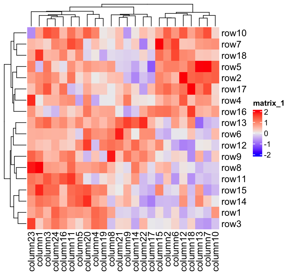
The title for the legend is taken from the “name” of the heatmap by default.
Each heatmap has a name which is like a unique identifier for the heatmap and
it is important when you have a list of heatmaps. In later chapters, you will
find the heatmap name is used for setting the “main heatmap” and is used for
decoration on heatmaps. If the name is not assigned, an internal name is
assigned to the heatmap in a form of matrix_%d. In the following examples in
this chapter, we give the name mat to the heatmap (for which you will see
the change of legend title in the next plot).
If you put Heatmap() inside a function or a for/if/while chunk, or the R script is run under command-line, you
won’t see the heatmap after executing Heatmap(). In this case, you need to
use draw() function explicitly as follows. We will explain this point in
more detail in Section 2.11.
for(...) {
    ht = Heatmap(mat)
    draw(ht)
}
2.1 Colors
For heatmap visualization, colors are the major representation of the data
matrix. In most cases, the heatmap visualizes a matrix with continuous numeric
values. In this case, users should provide a color mapping function. A color
mapping function should accept a vector of values and return a vector of
corresponding colors. Users should always use circlize::colorRamp2()
function to generate the color mapping function in Heatmap(). The
two arguments for colorRamp2() is a vector of break values and a vector of
corresponding colors. colorRamp2() linearly interpolates colors in every
interval through LAB color space. Also using colorRamp2() helps to generate
a legend with proper tick marks.
In following example, values between -2 and 2 are linearly interpolated to get corresponding colors, values larger than 2 are all mapped to red and values less than -2 are all mapped to green.
## [1] "#00FF00FF" "#00FF00FF" "#B1FF9AFF" "#FFFFFFFF" "#FF9E81FF" "#FF0000FF"
## [7] "#FF0000FF"
Heatmap(mat, name = "mat", col = col_fun)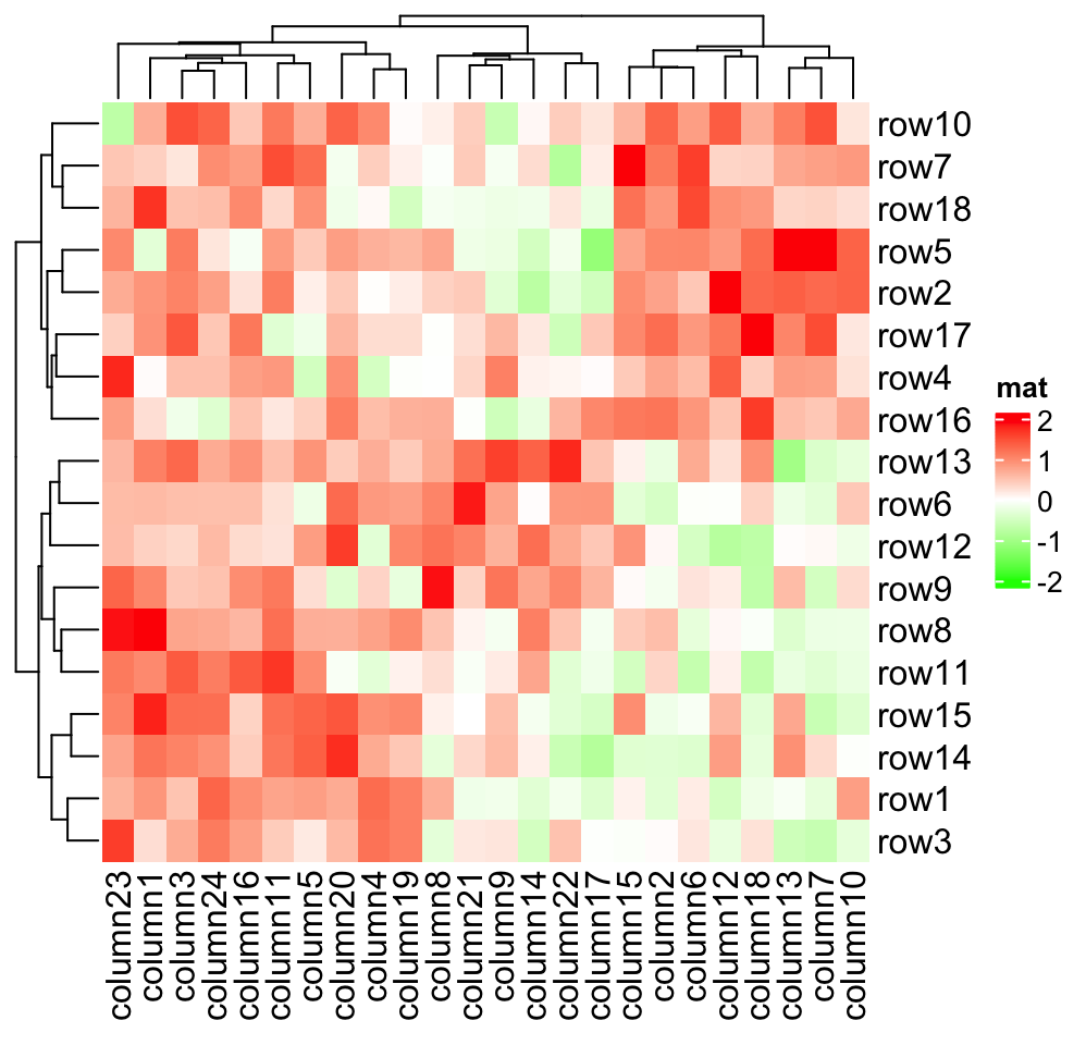
As you can see, the color mapping function exactly maps negative values to green and positive values to red, even when the distribution of negative values and positive values are not centric to zero. Also this color mapping function is not affected by outliers. In following plot, the clustering is heavily affected by the outlier (see the dendrogram) but not the color mapping.
mat2 = mat
mat2[1, 1] = 100000
Heatmap(mat2, name = "mat", col = col_fun,
    column_title = "a matrix with outliers")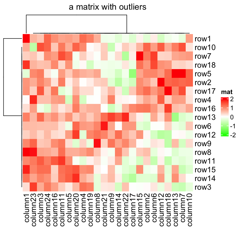
More importantly, colorRamp2() makes colors in multiple heatmaps comparible
if they are set with a same color mapping function. In following three
heatmaps, a same color always corresponds to a same value.
Heatmap(mat, name = "mat", col = col_fun, column_title = "mat")
Heatmap(mat/4, name = "mat", col = col_fun, column_title = "mat/4")
Heatmap(abs(mat), name = "mat", col = col_fun, column_title = "abs(mat)")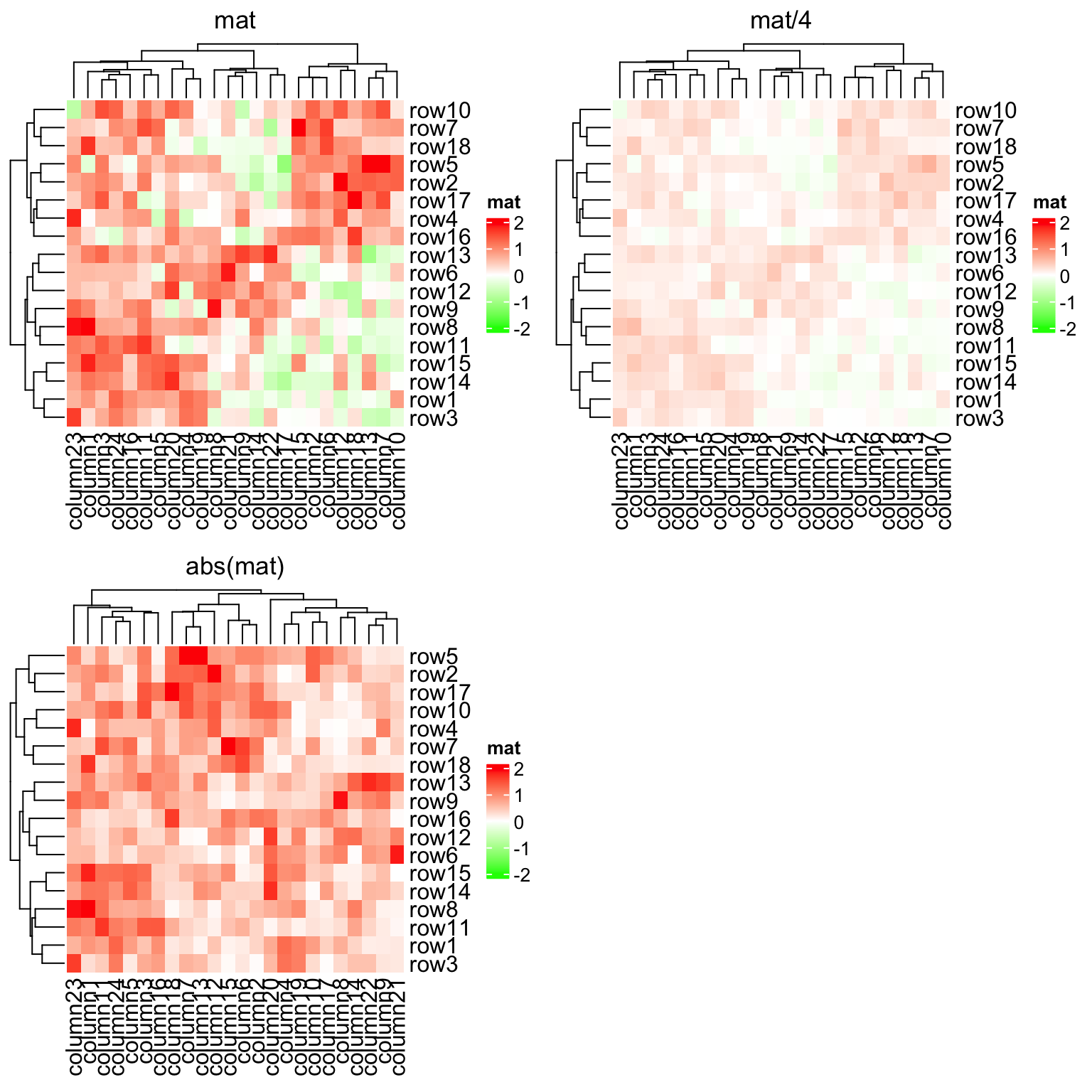
If the matrix is continuous, you can also simply provide a vector of colors
and colors will be linearly interpolated. But remember this method is not
robust to outliers because the mapping starts from the minimal value in the
matrix and ends with the maximal value. Following color mapping setting is
identical to colorRamp2(seq(min(mat), max(mat), length = 10), rev(rainbow(10))).
Heatmap(mat, name = "mat", col = rev(rainbow(10)),
    column_title = "set a color vector for a continuous matrix")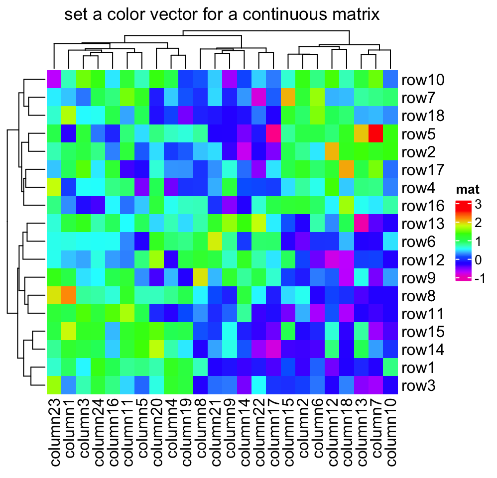
If the matrix contains discrete values (either numeric or character), colors
should be specified as a named vector to make it possible for the mapping from
discrete values to colors. If there is no name for the color vector, the order of
colors corresponds to the order of unique(mat). Note now the legend is
generated from the color mapping vector and it is a “discrete legend.”
In the following example, we set colors for a discrete numeric matrix. You don’t need to convert it to a character matrix, just set the numbers as “names” of the color vector.
discrete_mat = matrix(sample(1:4, 100, replace = TRUE), 10, 10)
colors = structure(1:4, names = c("1", "2", "3", "4")) # black, red, green, blue
Heatmap(discrete_mat, name = "mat", col = colors,
    column_title = "a discrete numeric matrix")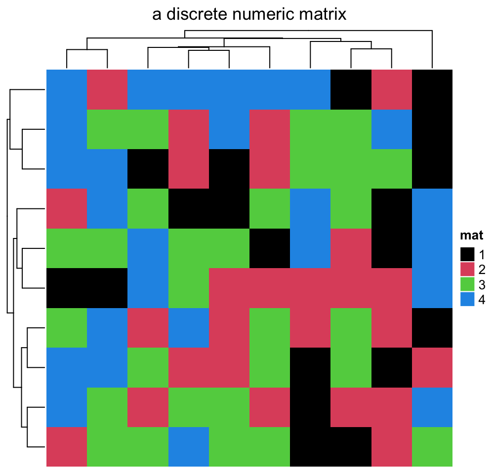
For a character matrix, it is straightforward.
discrete_mat = matrix(sample(letters[1:4], 100, replace = TRUE), 10, 10)
colors = structure(1:4, names = letters[1:4])
Heatmap(discrete_mat, name = "mat", col = colors,
    column_title = "a discrete character matrix")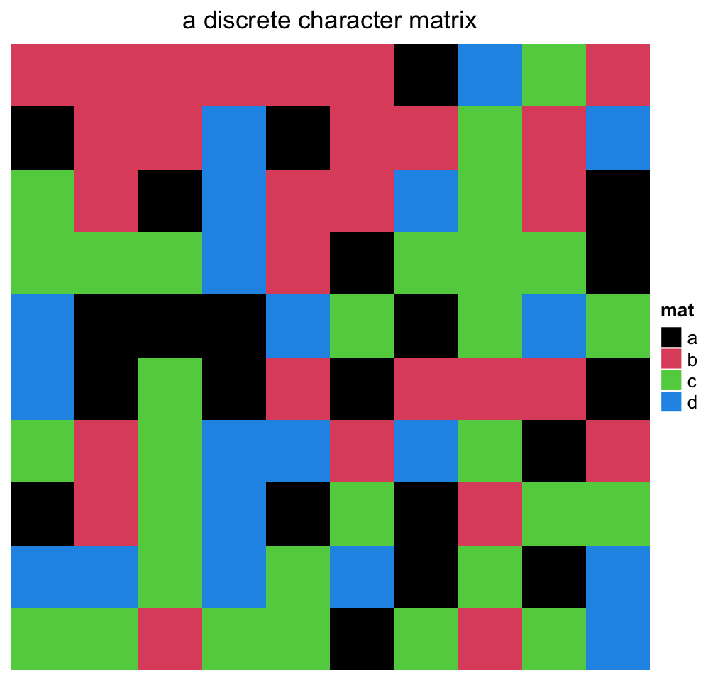
As you can see in the two examples above, for the numeric matrix (no matter the color is continuous mapping or discrete mapping), by default clustering is applied on both dimensions, while for character matrix, clustering is turned off (but you can still cluster a character matrix if you provide a proper distance metric for two character vectors, see example in Section 2.3.1).
NA is allowed in the matrix. You can control the color of NA by na_col
argument (by default it is grey for NA). A matrix that contains NA can
be clustered by Heatmap() as long as there is no NA distances between
any of the rows or columns respectively. Usually these cases correspond to
sparse matrices (filled with a lot of NA values), and indicate that the
unknown values should be predicted via other methods first.
Note the NA value is not presented in the legend.
mat_with_na = mat
na_index = sample(c(TRUE, FALSE), nrow(mat)*ncol(mat), replace = TRUE, prob = c(1, 9))
mat_with_na[na_index] = NA
Heatmap(mat_with_na, name = "mat", na_col = "black",
    column_title = "a matrix with NA values")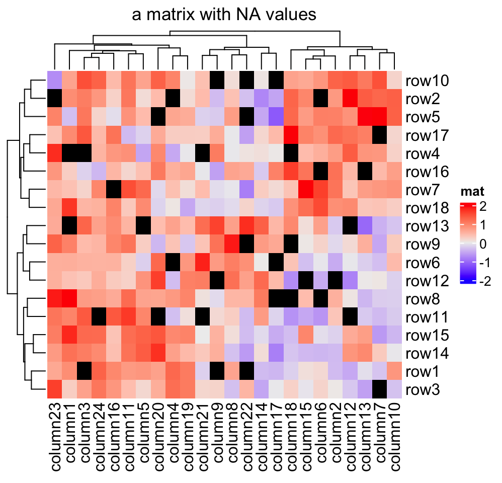
Color space is important for interpolating colors. By default, colors are
linearly interpolated in LAB color
space, but you can select the
color space in colorRamp2() function. Compare following two plots. Can you
see the difference?
f1 = colorRamp2(seq(min(mat), max(mat), length = 3), c("blue", "#EEEEEE", "red"))
f2 = colorRamp2(seq(min(mat), max(mat), length = 3), c("blue", "#EEEEEE", "red"), space = "RGB")
Heatmap(mat, name = "mat1", col = f1, column_title = "LAB color space")
Heatmap(mat, name = "mat2", col = f2, column_title = "RGB color space")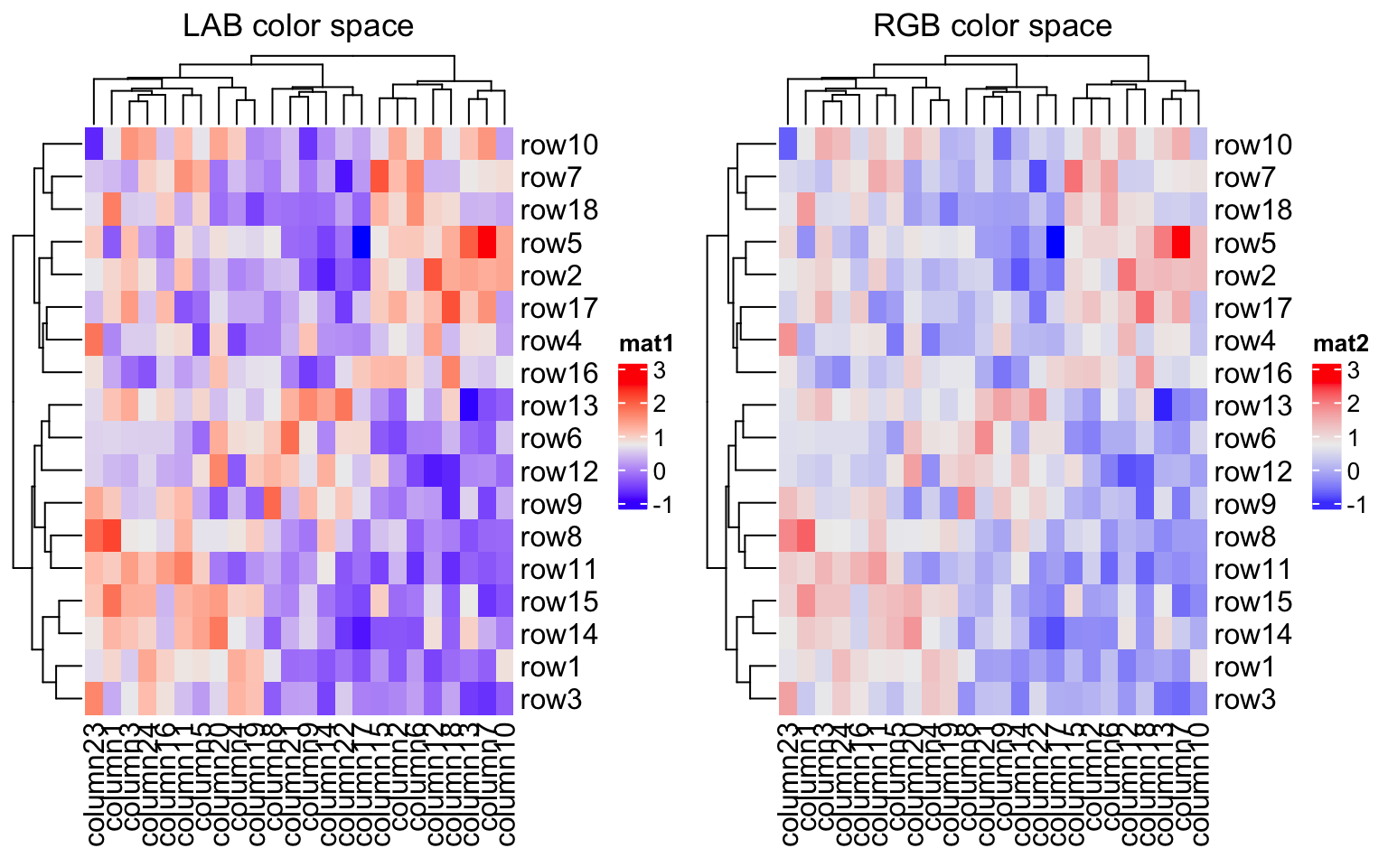
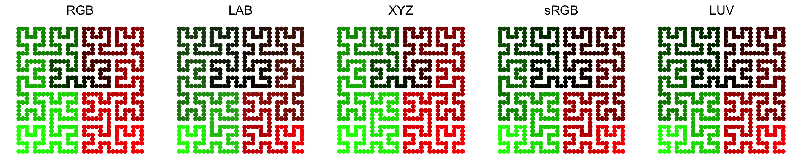
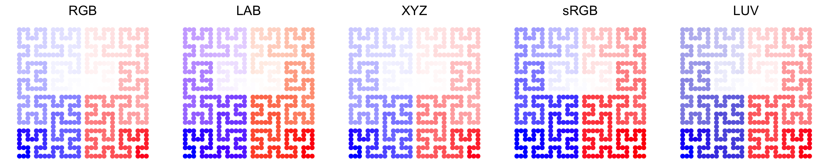
In following plots, corresponding values change evenly on the folded lines, you can see how colors change under different color spaces (top plots: green-black-red, bottom plots: blue-white-red. The plot is made by HilbertCurve package).
Last but not the least, colors for the heatmap borders can be set by the
border/border_gp and rect_gp arguments. border/border_gp controls
the global border of the heatmap body and rect_gp controls the border of the
grids/cells in the heatmap.
The value of border can be logical (TRUE corresponds to black) or a
character of color (e.g. red). The use for border argument is only for historical
reason, here you can also set border_gp argument which should be a gpar object.
rect_gp is a gpar object which means you can only set it by
grid::gpar(). Since the filled color is already controlled by the heatmap
color mapping, you can only set the col/lwd/lty parameters in gpar() to control the
border of the heatmap grids.
Heatmap(mat, name = "mat", border_gp = gpar(col = "black", lty = 2),
    column_title = "set heatmap borders")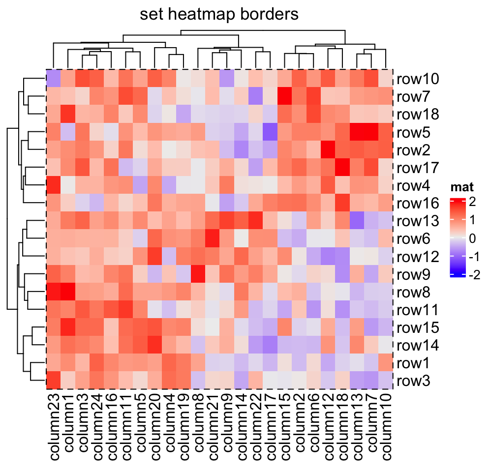
Heatmap(mat, name = "mat", rect_gp = gpar(col = "white", lwd = 2),
    column_title = "set cell borders")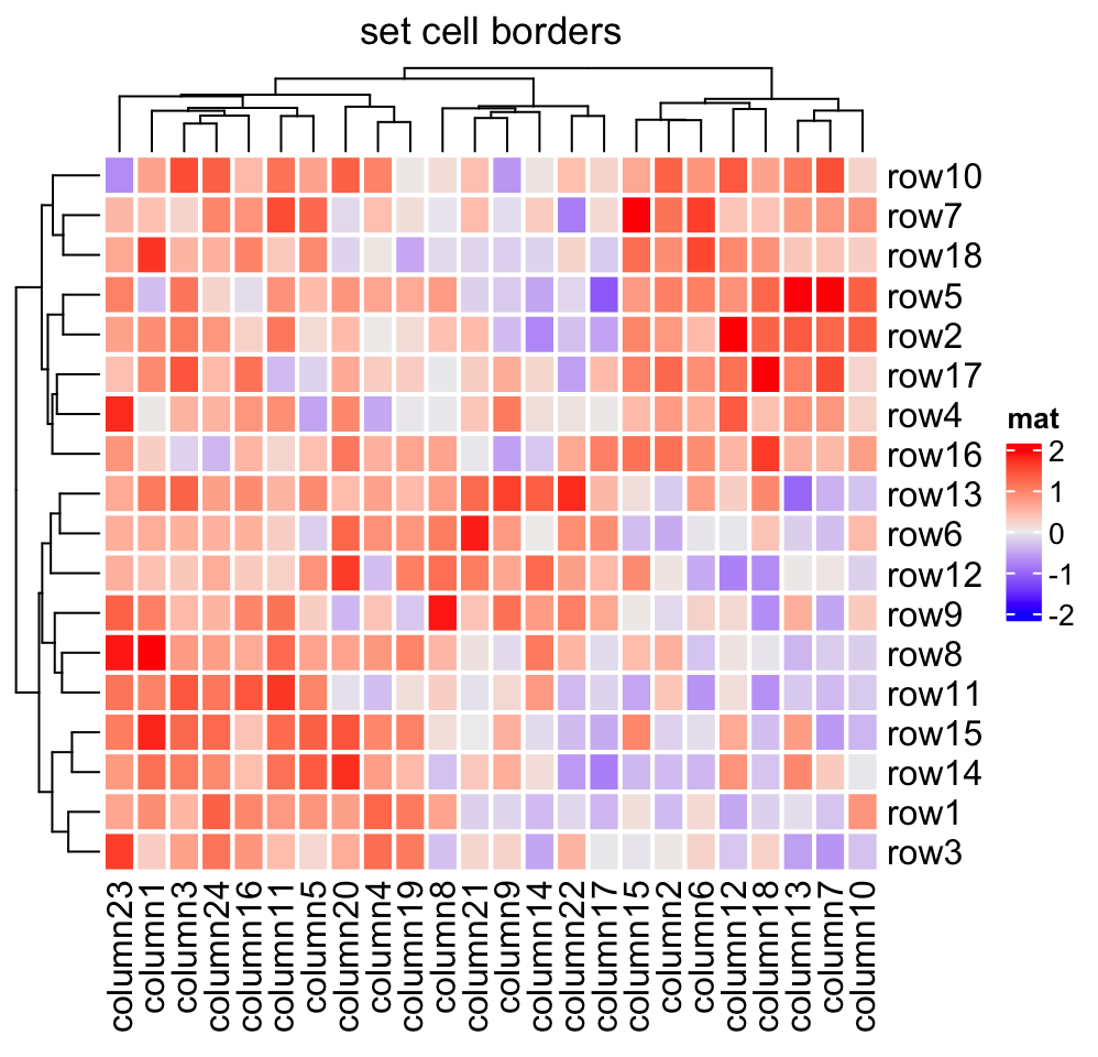
If col is not set, the default color mapping by Heatmap() is designed with
trying to be as convinient and meaningful as possible. Following are the rules
for the default color mapping (by ComplexHeatmap:::default_col()):
- If the values are characters, the colors are generated by
circlize::rand_color(). - If the values are from the heatmap annotation and are numeric, colors are mapped between white and one random color by linearly interpolating to the mininum and maxinum.
- If the values are from the matrix (let’s denote it as \(M\)):
- If the fraction of positive values in \(M\) is between 25% and 75%, colors are mapped to blue, white and red by linearly interpolating to \(-q\), 0 and \(q\), where \(q\) is the maximum of \(|M|\) if the number of unique values is less than 100, or \(q\) is the 99th percentile of \(|M|\) if there are more than 100 values in teh matrix. This color mapping is centric to zero.
- Or else the colors are mapped to blue, white and red by linearly interpolating to \(q_1\), \((q_1 + q_2)/2\) and \(q_2\), where \(q_1\) and \(q_2\) are mininum and maxinum if the number of unique values is \(M\) is less than 100. If there are more than 100 values in the matrix, \(q_1\) is the 1st percentile and \(q_2\) is the 99th percentile in \(M\).
rect_gp allows a non-standard parameter type. If it is set to "none",
the clustering is still applied but nothing in drawn on the heatmap body. The
customized graphics on heatmap body can be later added via a self-defined cell_fun
or layer_fun (explained in Section 2.9).
Heatmap(mat, name = "mat", rect_gp = gpar(type = "none"),
    column_title = "nothing is drawn in the heatmap body")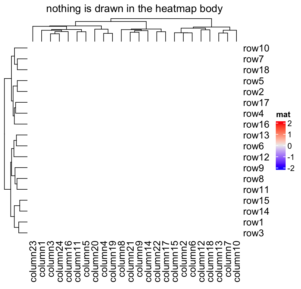
2.2 Titles
The title of the heatmap basically tells what the plot is about. In ComplexHeatmap package, you can set heatmap title either by the row or/and by the column. Note at a same time you can only put e.g. column title either on the top or at the bottom of the heatmap.
The graphic parameters can be set by row_title_gp and column_title_gp
respectively. Please remember you should use gpar() to specify graphics
parameters.
Heatmap(mat, name = "mat", column_title = "I am a column title",
    row_title = "I am a row title")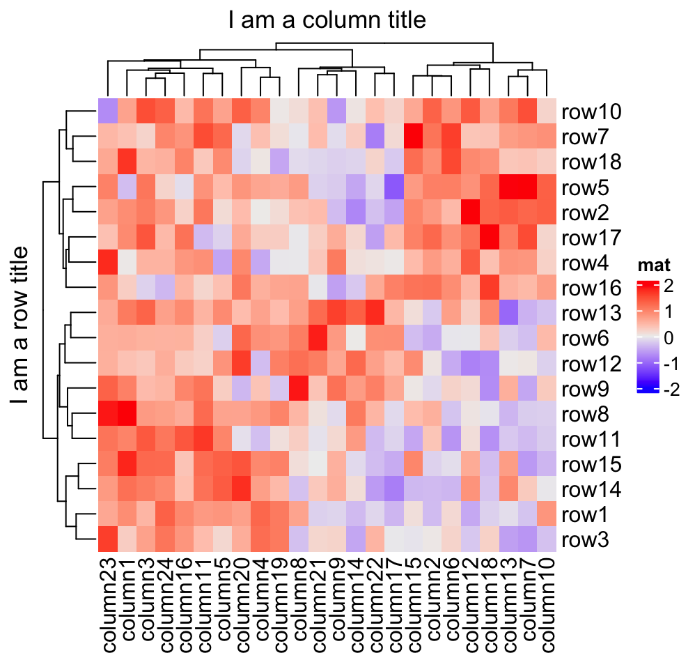
Heatmap(mat, name = "mat", column_title = "I am a column title at the bottom",
    column_title_side = "bottom")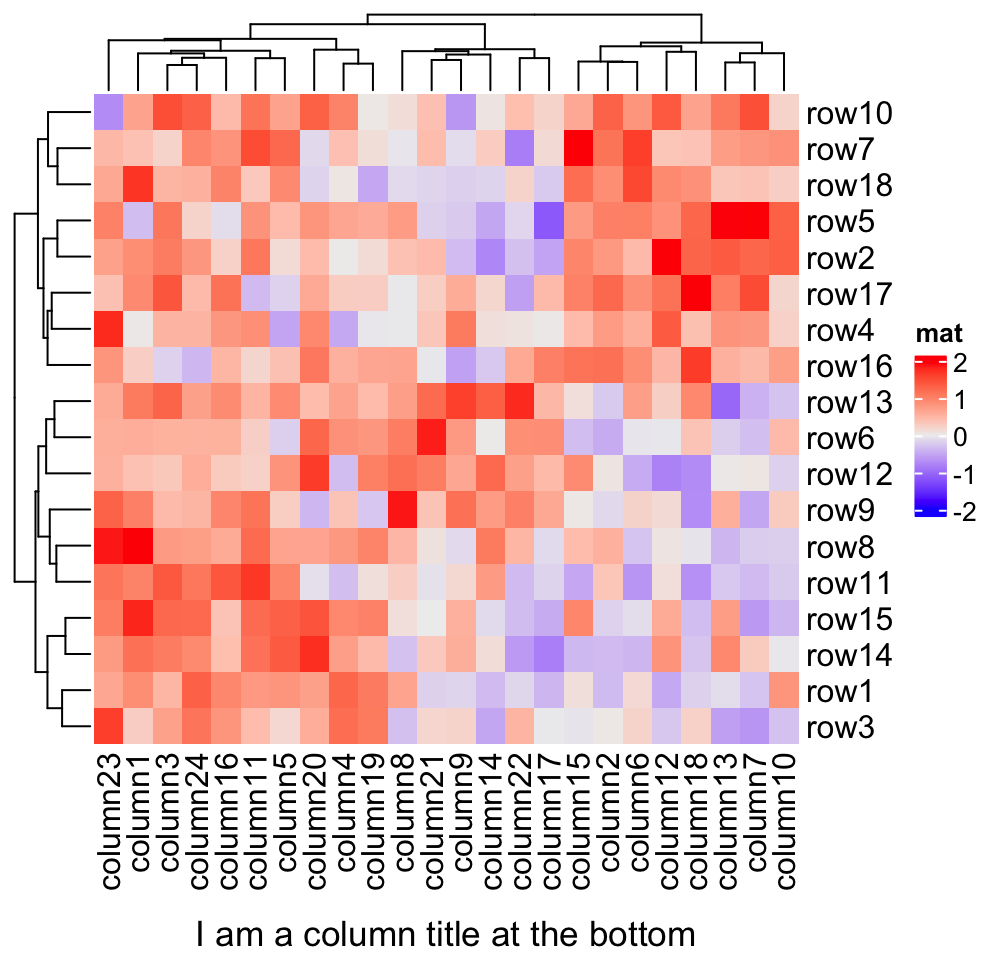
Heatmap(mat, name = "mat", column_title = "I am a big column title",
    column_title_gp = gpar(fontsize = 20, fontface = "bold"))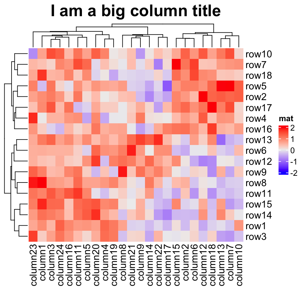
Rotations for titles can be set by row_title_rot and column_title_rot, but
only horizontal and vertical rotations are allowed.
Heatmap(mat, name = "mat", row_title = "row title", row_title_rot = 0)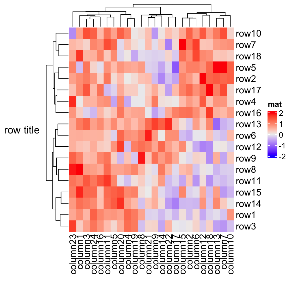
Row or column title supports as a template which is used when rows or columns are split in the heatmap (because there will be multiple row/column titles). This functionality is introduced in Section 2.7. A quick example would be:
# code only for demonstration
# row title would be cluster_1 and cluster_2
Heatmap(mat, name = "mat", row_km = 2, row_title = "cluster_%s")
You can set fill parameter in row_title_gp and column_title_gp to set
the background color of titles. Since col in e.g. row_title_gp controls the
color of text, border is used to control the color of the background border.
Heatmap(mat, name = "mat", column_title = "I am a column title",
    column_title_gp = gpar(fill = "red", col = "white", border = "blue"))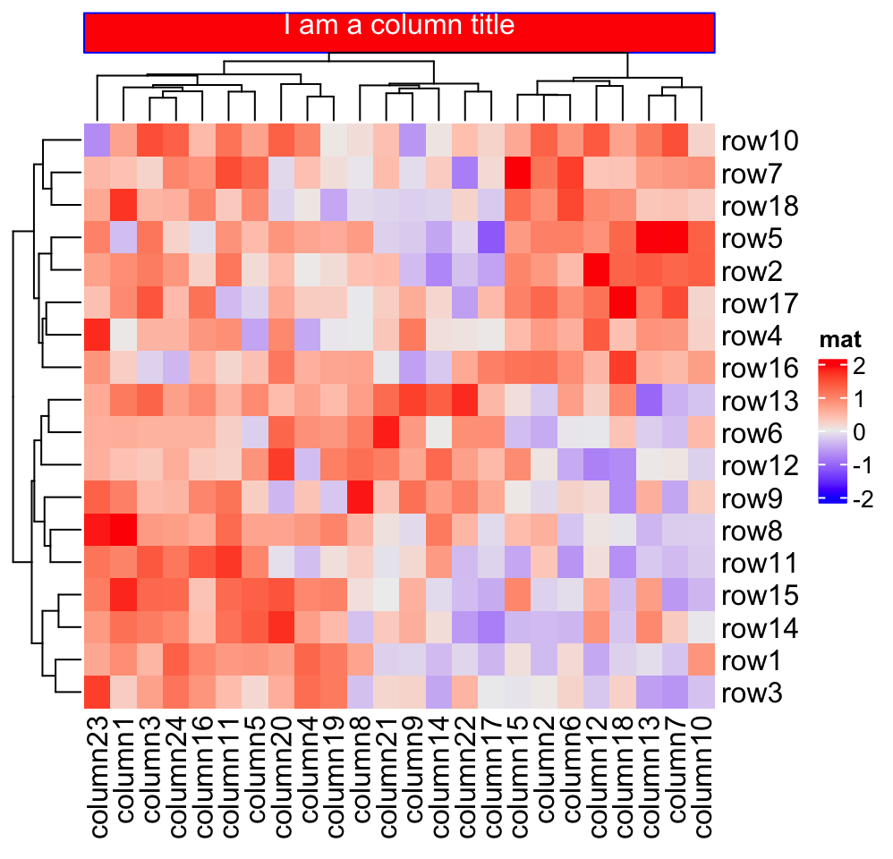
You might have found there is no space on the top of the column title when the background
is colored. This is mainly for being consistent to the figure titles of ggplot2 figures (when you make a multiple-panel figure mixed
with ComplexHeatmap and ggplot2 plots).
This can be adjusted by setting the global parameter ht_opt$TITLE_PADDING.
The use for ht_opt() will be introduced in Section 4.13.
ht_opt$TITLE_PADDING = unit(c(8.5, 8.5), "points")
Heatmap(mat, name = "mat", column_title = "I am a column title",
    column_title_gp = gpar(fill = "red", col = "white", border = "blue"))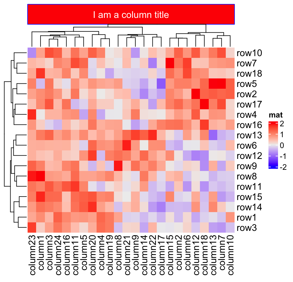
ht_opt(RESET = TRUE)Title can be set as mathematical formulas.
Heatmap(mat, name = "mat",
column_title = expression(hat(beta) == (X^t * X)^{-1} * X^t * y)) 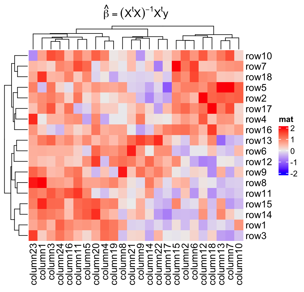
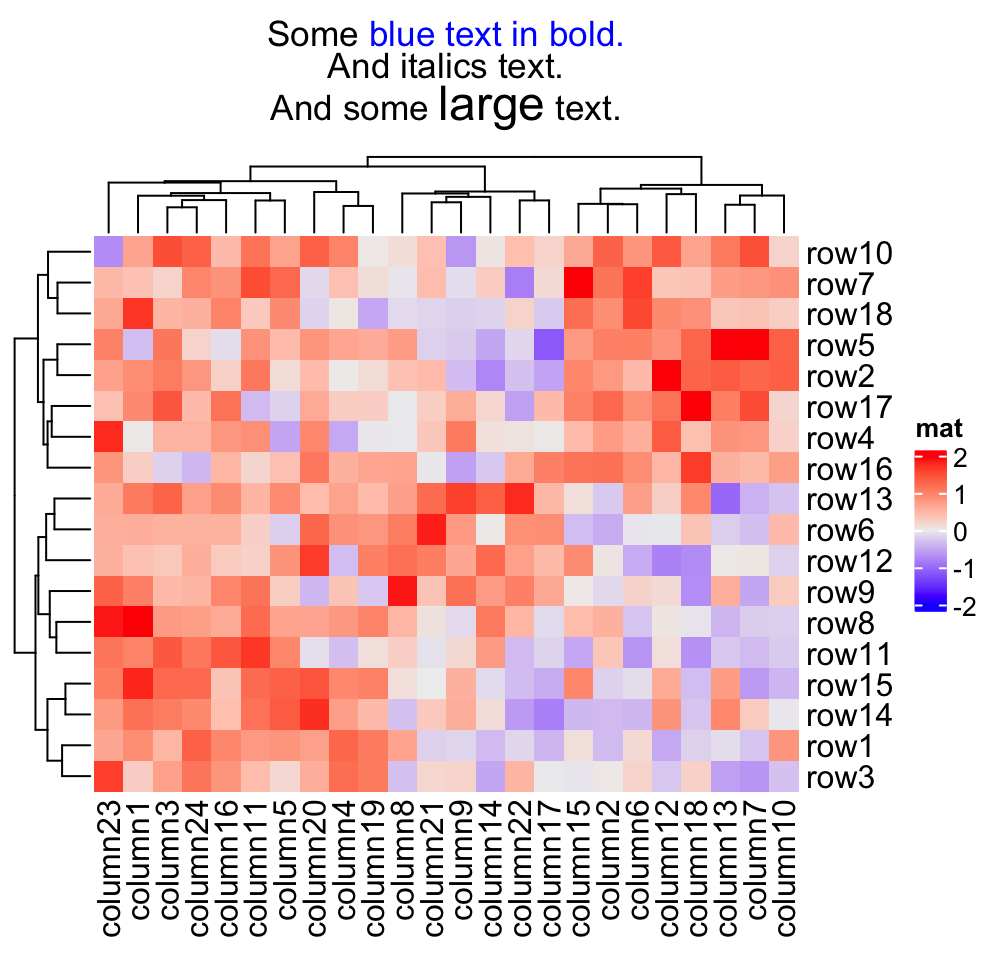
More complicated text can be drawn as the heatmap title by using the gridtext package. Following plot fives a quick example. See Section 10.3.1 for more examples.
Heatmap(mat, name = "mat",
    column_title = gt_render(
        paste0("Some <span style='color:blue'>blue text **in bold.**</span><br>",
            "And *italics text.*<br>And some ",
            "<span style='font-size:18pt; color:black'>large</span> text."),
        r = unit(2, "pt"),
        padding = unit(c(2, 2, 2, 2), "pt")
    )
)
2.3 Clustering
Clustering might be the key component of heatmap visualization. In ComplexHeatmap package, hierarchical clustering is supported with great flexibility. You can specify the clustering either by:
- a pre-defined distance method (e.g.
"euclidean"or"pearson"), - a distance function,
- a object that already contains clustering (a
hclustordendrogramobject or object that can be coerced todendrogramclass), - a clustering function.
It is also possible to render the dendrograms with different colors and styles
for different nodes and branches for better revealing structures of the dendrogram (e.g.
by dendextend::color_branches()).
First, there are general settings for the clustering, e.g. whether to apply clustering or show dendrograms, the side of the dendrograms and heights of the dendrograms.
Heatmap(mat, name = "mat", cluster_rows = FALSE) # turn off row clustering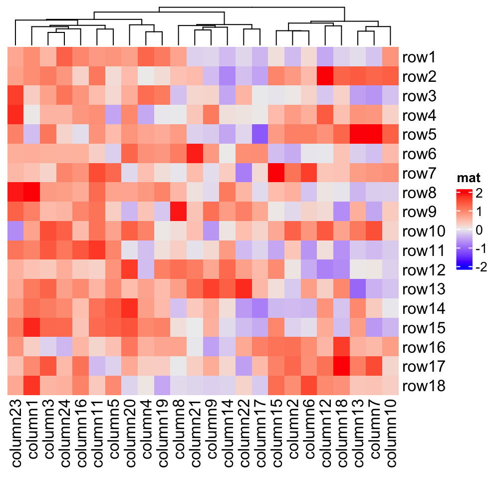
Heatmap(mat, name = "mat", show_column_dend = FALSE) # hide column dendrogram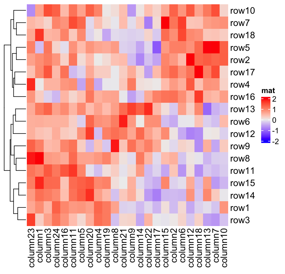
Heatmap(mat, name = "mat", row_dend_side = "right", column_dend_side = "bottom")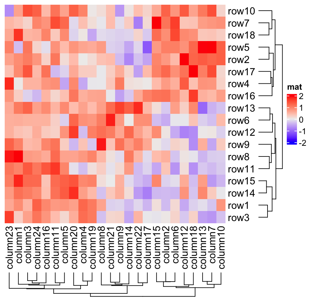
Heatmap(mat, name = "mat", column_dend_height = unit(4, "cm"),
    row_dend_width = unit(4, "cm"))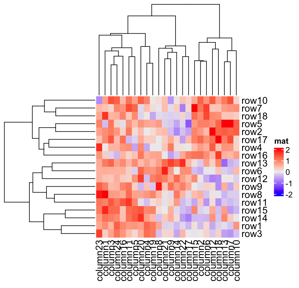
2.3.1 Distance methods
Hierarchical clustering is performed in two steps: calculate the distance matrix and apply clustering. There are three ways to specify distance metric for clustering:
- specify distance as a pre-defined option. The valid values are the supported
methods in
dist()function and in"pearson","spearman"and"kendall". The correlation distance is defined as1 - cor(x, y, method). All these built-in distance methods allowNAvalues. - a self-defined function which calculates distance from a matrix. The function should only contain one argument. Please note for clustering on columns, the matrix will be transposed automatically.
- a self-defined function which calculates distance from two vectors. The
function should only contain two arguments. Note this might be slow because
it is implemented by two nested
forloop.
Heatmap(mat, name = "mat", clustering_distance_rows = "pearson",
    column_title = "pre-defined distance method (1 - pearson)")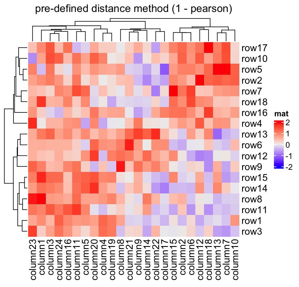
Heatmap(mat, name = "mat", clustering_distance_rows = function(m) dist(m),
    column_title = "a function that calculates distance matrix")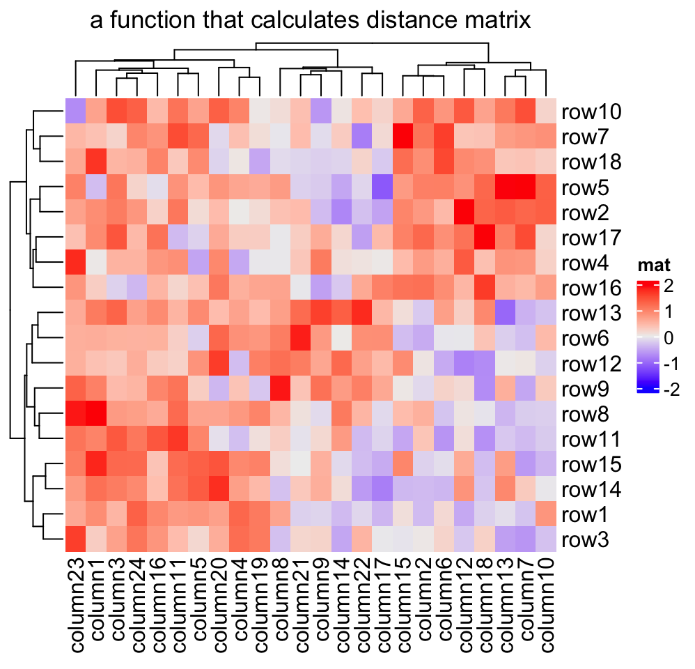
Heatmap(mat, name = "mat", clustering_distance_rows = function(x, y) 1 - cor(x, y),
    column_title = "a function that calculates pairwise distance")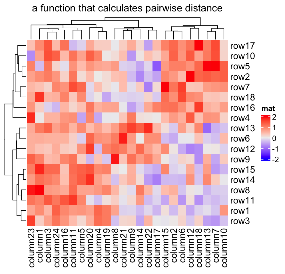
Based on these features, we can apply clustering which is robust to outliers based on the pairwise distance. Note here we set the color mapping function because we don’t want outliers affect the colors.
mat_with_outliers = mat
for(i in  1:10) mat_with_outliers[i, i] = 1000
robust_dist = function(x, y) {
    qx = quantile(x, c(0.1, 0.9))
    qy = quantile(y, c(0.1, 0.9))
    l = x > qx[1] & x < qx[2] & y > qy[1] & y < qy[2]
    x = x[l]
    y = y[l]
    sqrt(sum((x - y)^2))
}
We can compare the two heatmaps with or without the robust distance method:
Heatmap(mat_with_outliers, name = "mat",
    col = colorRamp2(c(-2, 0, 2), c("green", "white", "red")),
    column_title = "dist")
Heatmap(mat_with_outliers, name = "mat",
    col = colorRamp2(c(-2, 0, 2), c("green", "white", "red")),
    clustering_distance_rows = robust_dist,
    clustering_distance_columns = robust_dist,
    column_title = "robust_dist")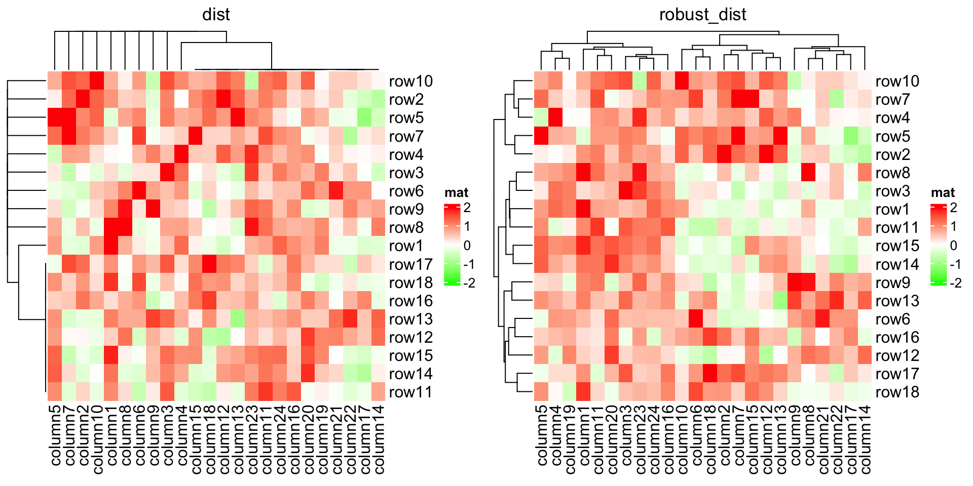
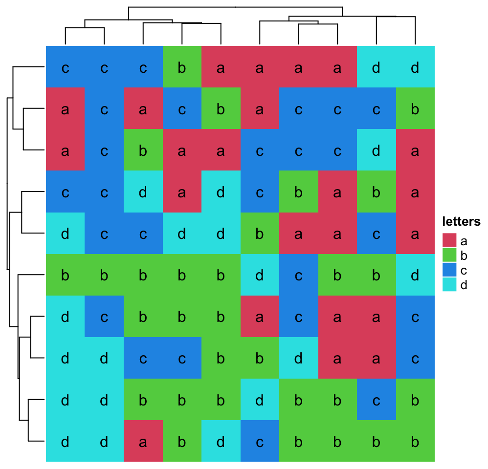
If there are proper distance methods (like methods in stringdist
package), you can also
cluster a character matrix. cell_fun argument will be introduced in Section
2.9.
mat_letters = matrix(sample(letters[1:4], 100, replace = TRUE), 10)
# distance in the ASCII table
dist_letters = function(x, y) {
    x = strtoi(charToRaw(paste(x, collapse = "")), base = 16)
    y = strtoi(charToRaw(paste(y, collapse = "")), base = 16)
    sqrt(sum((x - y)^2))
}
Heatmap(mat_letters, name = "letters", col = structure(2:5, names = letters[1:4]),
    clustering_distance_rows = dist_letters,
    clustering_distance_columns = dist_letters,
    cell_fun = function(j, i, x, y, w, h, col) { # add text to each grid
        grid.text(mat_letters[i, j], x, y)
    })
2.3.2 Clustering methods
Method to perform hierarchical clustering can be specified by
clustering_method_rows and clustering_method_columns. Possible methods are
those supported in hclust() function.
Heatmap(mat, name = "mat", clustering_method_rows = "single")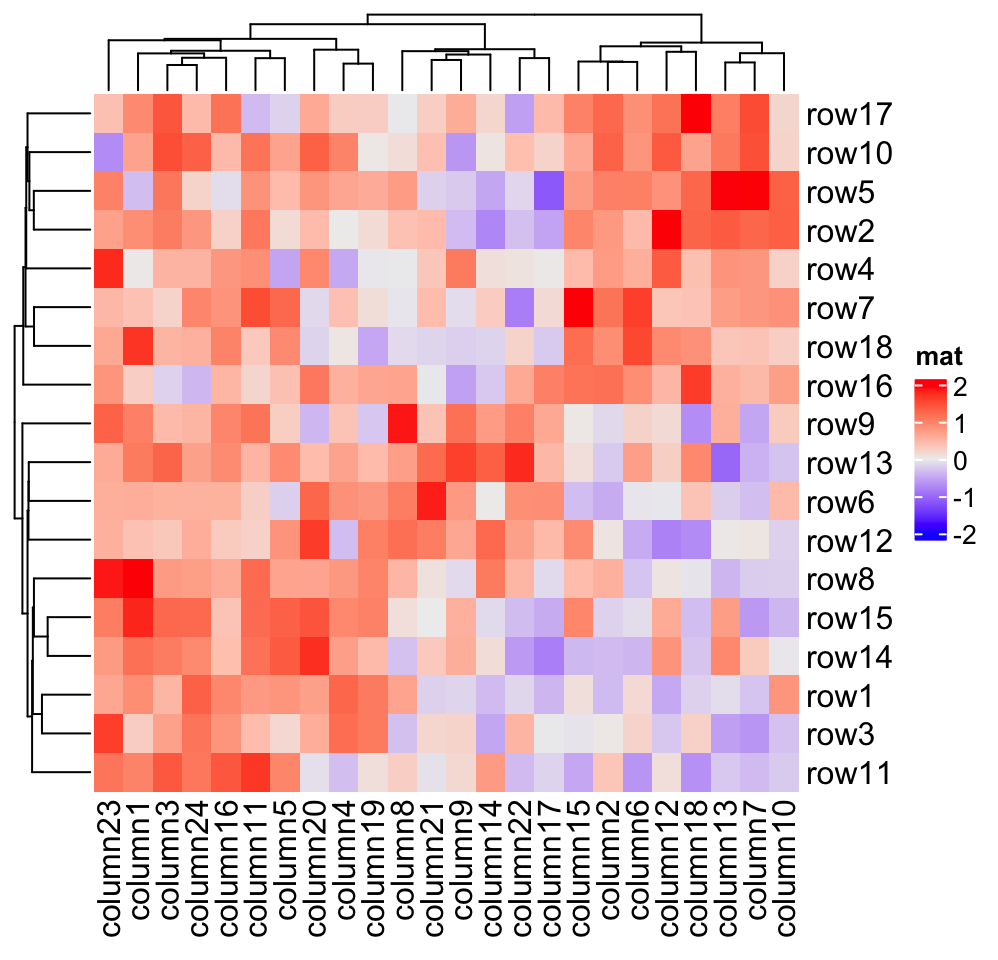
If you already have a clustering object or a function which directly returns a
clustering object, you can ignore the distance settings and set cluster_rows
or cluster_columns to the clustering objects or clustering functions. If it
is a clustering function, the only argument should be the matrix and it should
return a hclust or dendrogram object or a object that can be converted to
the dendrogram class.
In following example, we perform clustering with methods from cluster package either by a pre-calculated clustering object or a clustering function:
library(cluster)
Heatmap(mat, name = "mat", cluster_rows = diana(mat),
   cluster_columns = agnes(t(mat)), column_title = "clustering objects")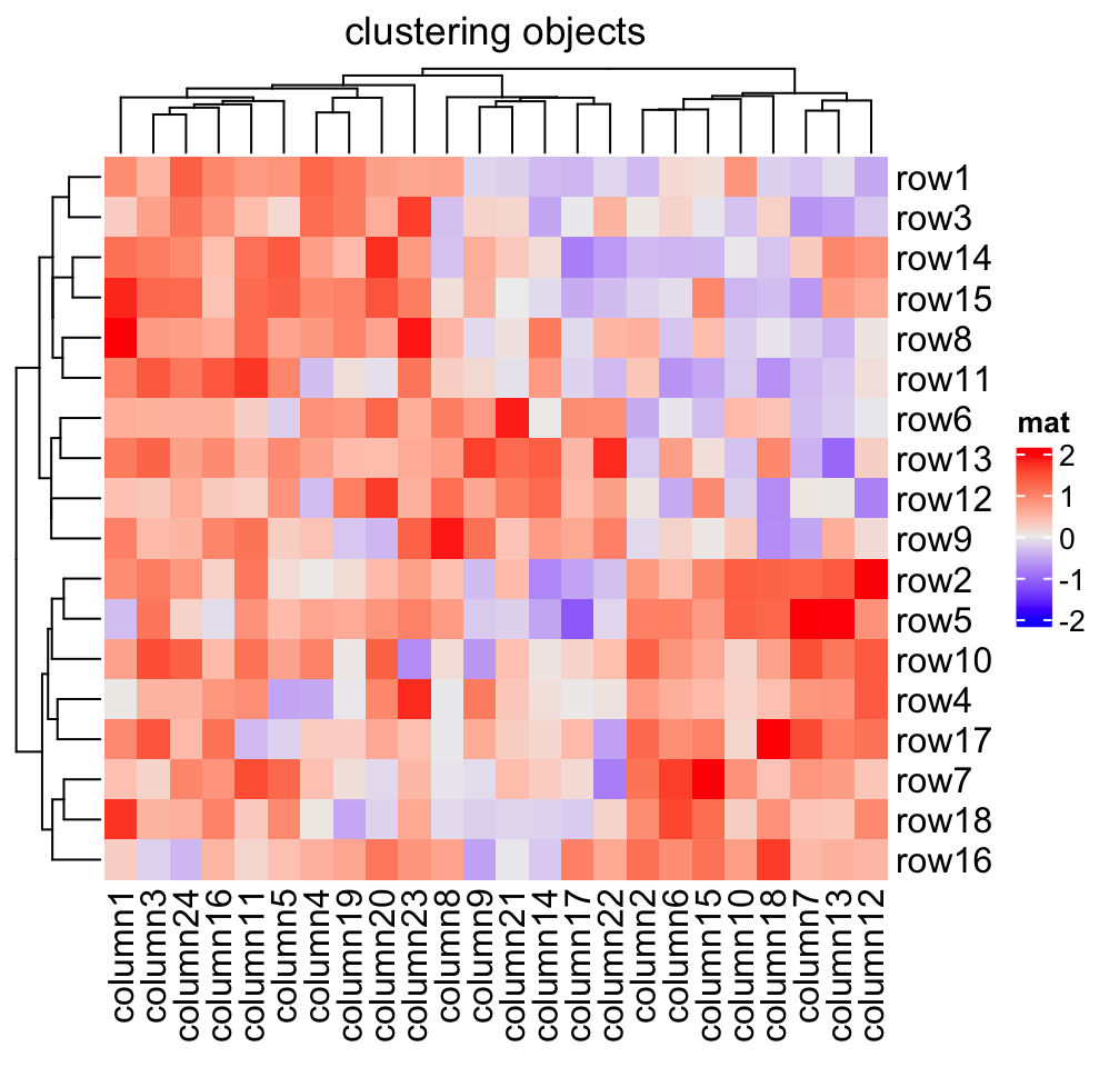
# if cluster_columns is set as a function, you don't need to transpose the matrix
Heatmap(mat, name = "mat", cluster_rows = diana,
   cluster_columns = agnes, column_title = "clustering functions")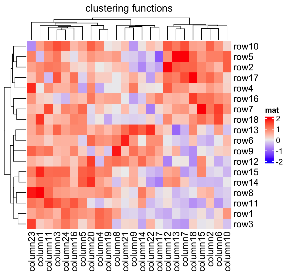
The last command is as same as :
# code only for demonstration
Heatmap(mat, name = "mat", cluster_rows = function(m) as.dendrogram(diana(m)),
    cluster_columns = function(m) as.dendrogram(agnes(m)),
    column_title = "clutering functions")
Please note, when cluster_rows is set as a function, the argument m is the
input mat itself, while for cluster_columns, m is the transpose of
mat.
fastcluster::hclust implements a faster version of hclust(). You can set
it to cluster_rows and cluster_columns to use the faster version of
hclust().
# code only for demonstration
fh = function(x) fastcluster::hclust(dist(x))
Heatmap(mat, name = "mat", cluster_rows = fh, cluster_columns = fh)
To make it more convinient to use the faster version of hclust() (assuming
you have many heatmaps to construct), it can be set as a global option. The
usage of ht_opt is introduced in Section
4.13.
# code only for demonstration
ht_opt$fast_hclust = TRUE
# now fastcluster::hclust is used in all heatmaps
This is one special scenario where you might already have a subgroup
classification for the matrix rows or columns, and you only want to perform
clustering for the features in the same subgroup. You
can split the heatmap by the subgroup variable (see Section
2.7), or you can use cluster_within_group() clustering
function to generate a special dendrogram.
group = kmeans(t(mat), centers = 3)$cluster
Heatmap(mat, name = "mat", cluster_columns = cluster_within_group(mat, group))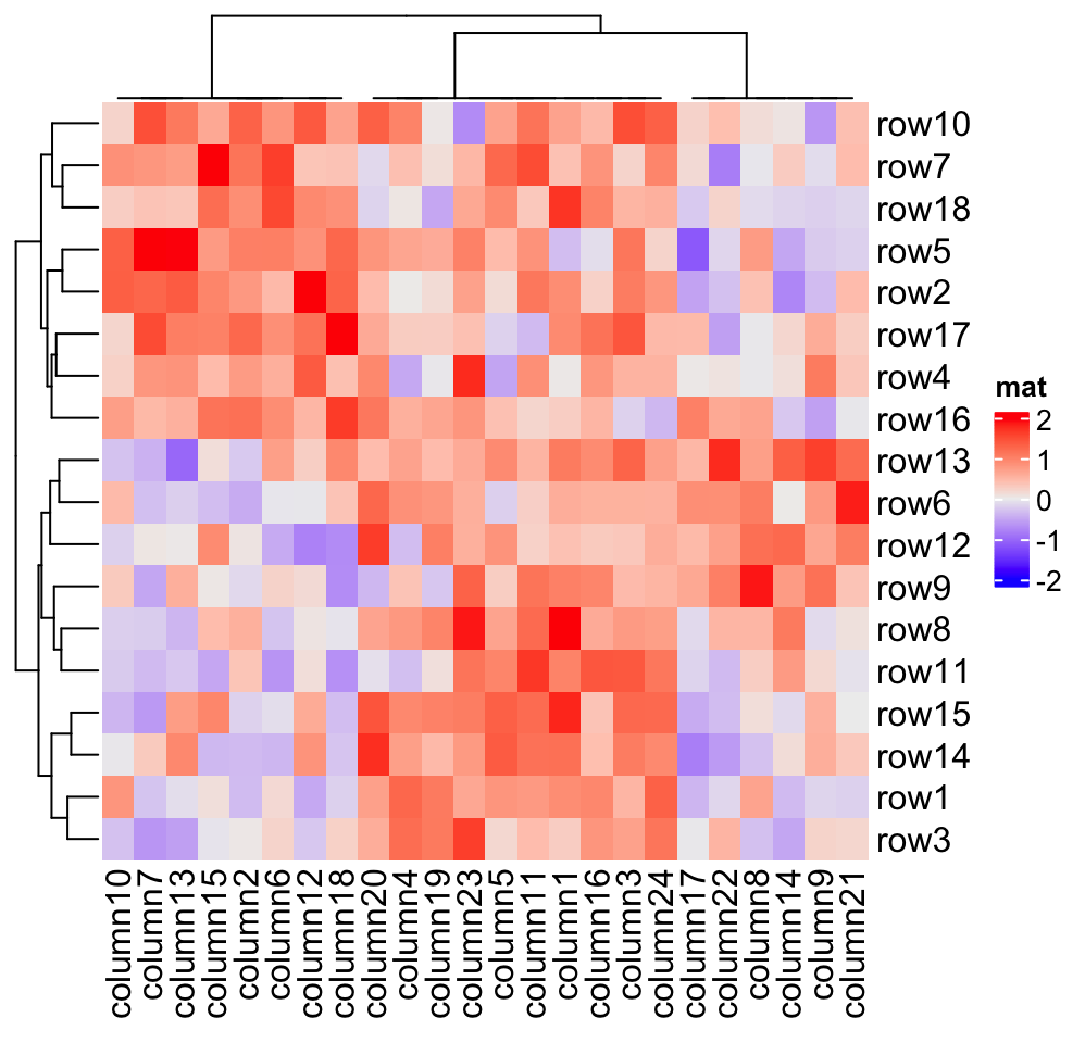
In above example, columns in a same group are still clustered, but the dendrogram is degenerated as a flat line. The dendrogram on columns shows the hierarchy of the groups.
2.3.3 Render dendrograms
If you want to render the dendrogram, normally you need to generate a
dendrogram object and render it through nodePar and edgePar parameter in
advance, then send it to the cluster_rows or cluster_columns argument.
You can render your dendrogram object by the dendextend package to make
a more customized visualization of the dendrogram.
library(dendextend)
row_dend = as.dendrogram(hclust(dist(mat)))
row_dend = color_branches(row_dend, k = 2) # `color_branches()` returns a dendrogram object
Heatmap(mat, name = "mat", cluster_rows = row_dend)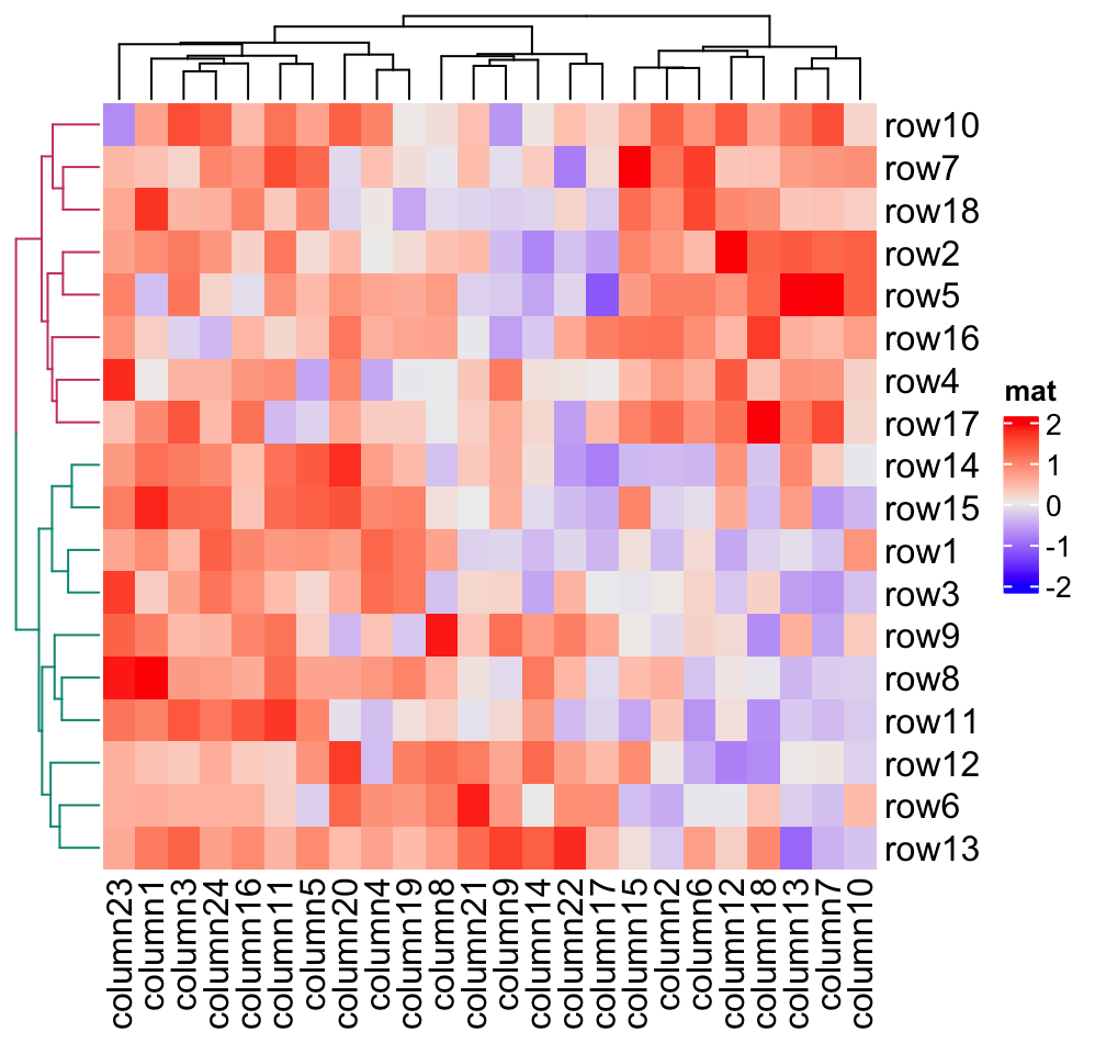
row_dend_gp and column_dend_gp control the global graphics setting for
dendrograms. Note e.g. graphics settings in row_dend will be overwritten by
row_dend_gp.
Heatmap(mat, name = "mat", cluster_rows = row_dend,
    row_dend_gp = gpar(col = "red"))
From version 2.5.6, you can also add graphics on the nodes of the dendrogram by setting
a proper nodePar.
row_dend = dendrapply(row_dend, function(d) {
    attr(d, "nodePar") = list(cex = 0.8, pch = sample(20, 1), col = rand_color(1))
    return(d)
})
Heatmap(mat, name = "mat", cluster_rows = row_dend, row_dend_width = unit(2, "cm"))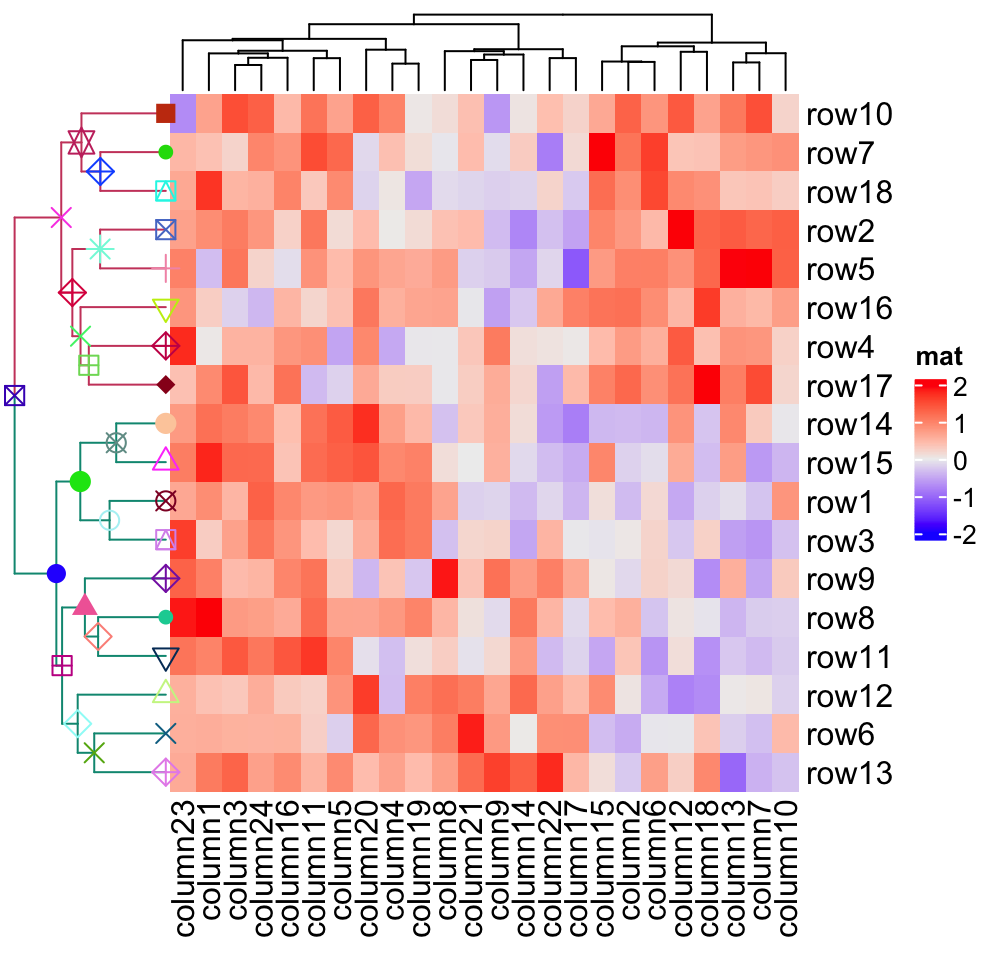
Currently, only points can be added on the nodes, however, if you have the need to add more types of graphics, especially the self-defined graphics, just send me a message and I will think about it.
2.3.4 Reorder dendrograms
In the Heatmap() function, dendrograms are reordered to make features with
larger difference more separated from each others (please refer to the
documentation of reorder.dendrogram()). Here the difference (or it is called
the weight) is measured by the row means if it is a row dendrogram or by the
column means if it is a column dendrogram. row_dend_reorder and
column_dend_reorder control whether to apply dendrogram reordering if the
value is set as logical. The two arguments also control the weight for the
reordering if they are set to numeric vectors (it will be sent to the wts
argument of reorder.dendrogram()). The reordering can be turned off by
setting e.g. row_dend_reorder = FALSE.
By default, dendrogram reordering is turned on if
cluster_rows/cluster_columns is set as logical value or a clustering
function. It is turned off if cluster_rows/cluster_columns is set as
clustering object.
Compare following two heatmaps:
m2 = matrix(1:100, nr = 10, byrow = TRUE)
Heatmap(m2, name = "mat", row_dend_reorder = FALSE, column_title = "no reordering")
Heatmap(m2, name = "mat", row_dend_reorder = TRUE, column_title = "apply reordering")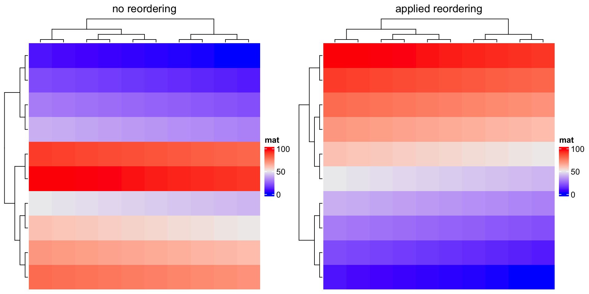
There are many other methods for reordering dendrograms, e.g. the dendsort
package. Basically, all these methods still return a dendrogram that has been
reordered, thus, we can firstly generate the row or column dendrogram based on
the data matrix, reorder it by a certain method, and assign it back to
cluster_rows or cluster_columns.
Compare following two reorderings on both dimensions. Can you tell which is better?
Heatmap(mat, name = "mat", column_title = "default reordering")

library(dendsort)
row_dend = dendsort(hclust(dist(mat)))
col_dend = dendsort(hclust(dist(t(mat))))
Heatmap(mat, name = "mat", cluster_rows = row_dend, cluster_columns = col_dend,
    column_title = "reorder by dendsort")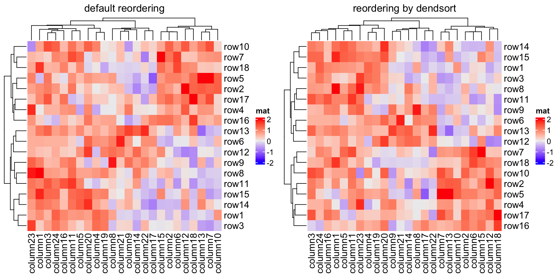
2.4 Set row and column orders
Clustering is used to adjust row orders and column orders of the heatmap, but
you can still set the order manually by row_order and column_order. If
e.g. row_order is set, row clustering is turned off by default.
Heatmap(mat, name = "mat",
    row_order = order(as.numeric(gsub("row", "", rownames(mat)))),
    column_order = order(as.numeric(gsub("column", "", colnames(mat)))),
    column_title = "reorder matrix")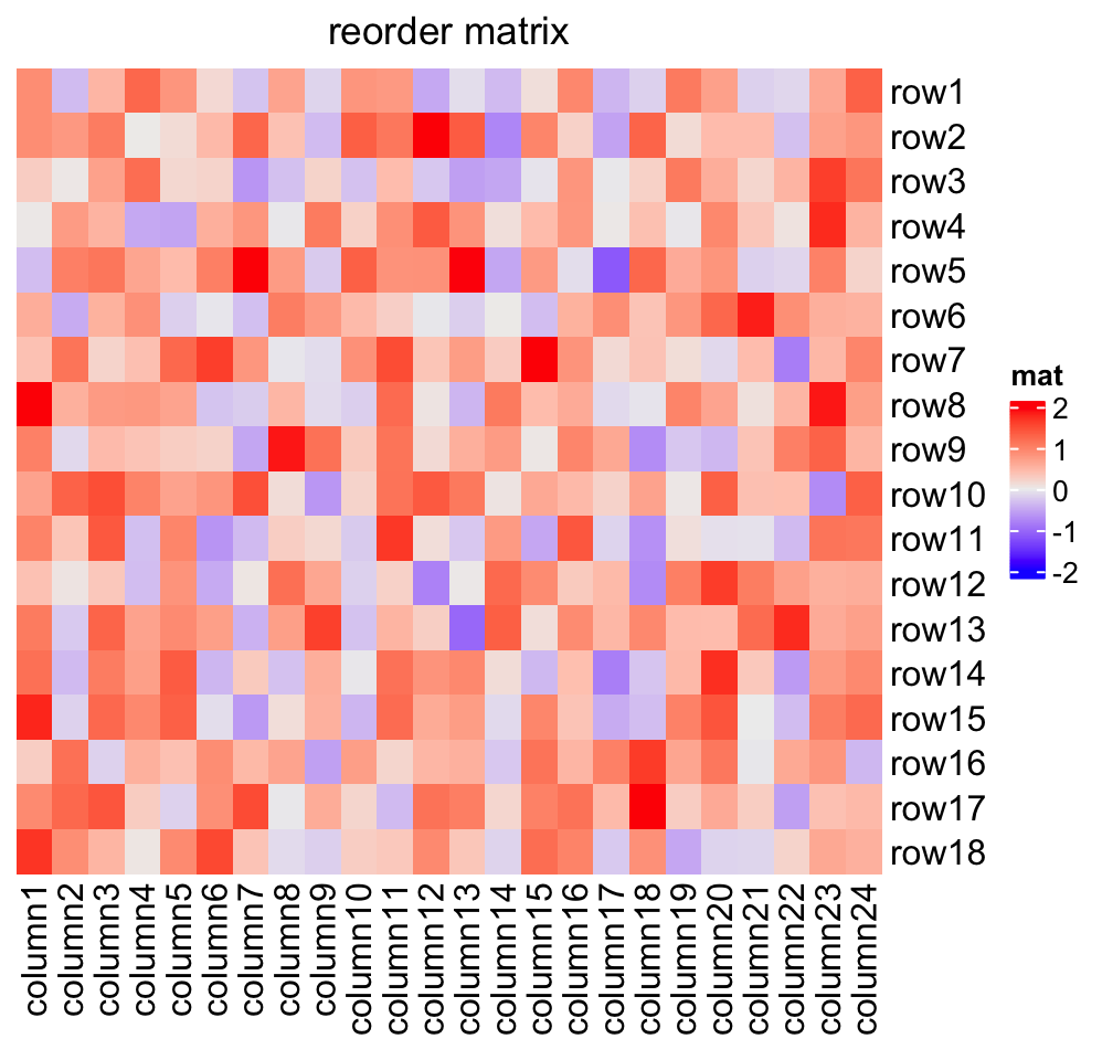
The orders can be character vectors if they are just shuffles of the matrix row names or column names.
Heatmap(mat, name = "mat", row_order = sort(rownames(mat)),
    column_order = sort(colnames(mat)),
    column_title = "reorder matrix by row/column names")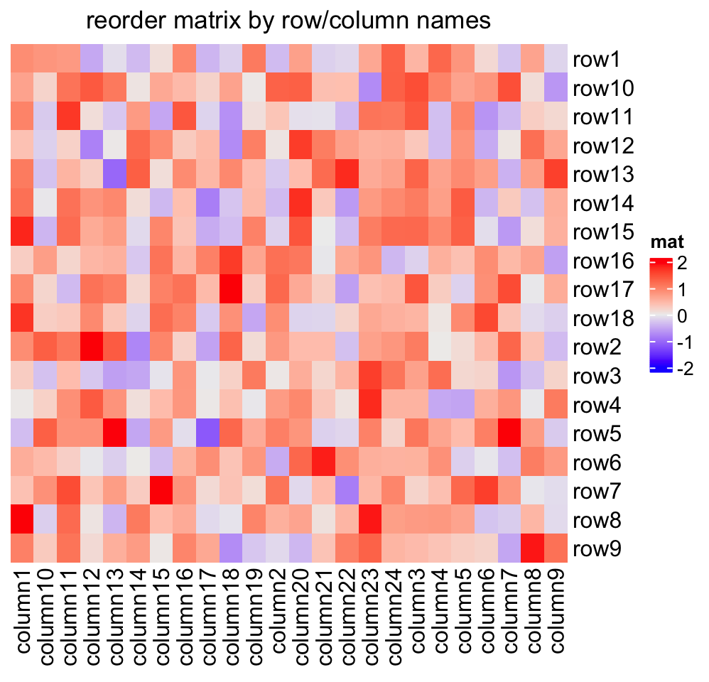
Note row_dend_reorder and row_order are two different things.
row_dend_reorder is applied on the dendrogram. For any node in the
dendrogram, rotating its two branches actually gives an identical dendrogram,
thus, reordering the dendrogram by automatically rotating sub-dendrogram at
every node can help to separate features further from each other which show
more difference. As a comparison, row_order is simply applied to the matrix
and normally dendrograms should be turned off.
2.5 Seriation
Seriation is an interesting technique for ordering the matrix (see this
interesting post: http://nicolas.kruchten.com/content/2018/02/seriation/). The
powerful seriation
package
implements quite a lot of methods for seriation. Since it is easy to extract
row orders and column orders from the object returned by the core function
seriate() from seriation package, they can be directly assigned to
row_order and column_order to make the heatmap.
The first example demonstrates directly applying seriate() on the matrix.
Since the "BEA_TSP" method only allows a non-negative matrix, we modify the
matrix to max(mat) - mat.
library(seriation)
o = seriate(max(mat) - mat, method = "BEA_TSP")
Heatmap(max(mat) - mat, name = "mat",
    row_order = get_order(o, 1), column_order = get_order(o, 2),
    column_title = "seriation by BEA_TSP method")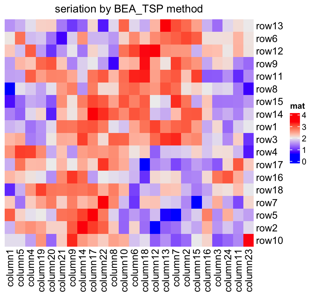
Or you can apply seriate() to the distance matrix. Now the order for rows
and columns needs to be calcualted separatedly because the distance matrix
needs to be calculated separatedly for columns and rows.
o1 = seriate(dist(mat), method = "TSP")
o2 = seriate(dist(t(mat)), method = "TSP")
Heatmap(mat, name = "mat", row_order = get_order(o1), column_order = get_order(o2),
    column_title = "seriation from the distance matrix")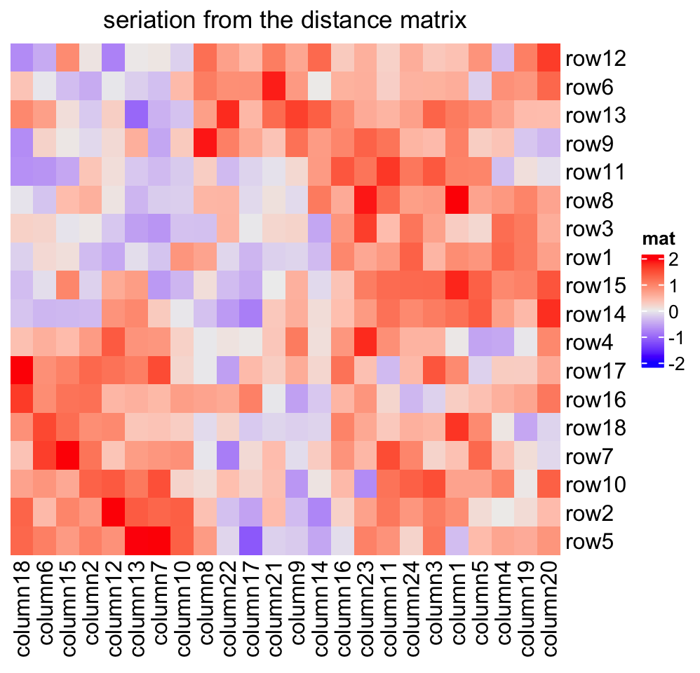
Some seriation methods also contain the hierarchical clustering information. Let’s try:
o1 and o2 are actually mainly composed of hclust objects:
class(o1[[1]])## [1] "ser_permutation_vector" "hclust"And the orders are the same by using hclust$order or get_order().
o1[[1]]$order## [1] 5 2 4 17 16 7 18 10 14 15 1 3 8 11 9 13 6 12
# should be the same as the previous one
get_order(o1)
## [1] 5 2 4 17 16 7 18 10 14 15 1 3 8 11 9 13 6 12And we can add the dendrograms to the heatmap.
Heatmap(mat, name = "mat", cluster_rows = as.dendrogram(o1[[1]]),
    cluster_columns = as.dendrogram(o2[[1]]))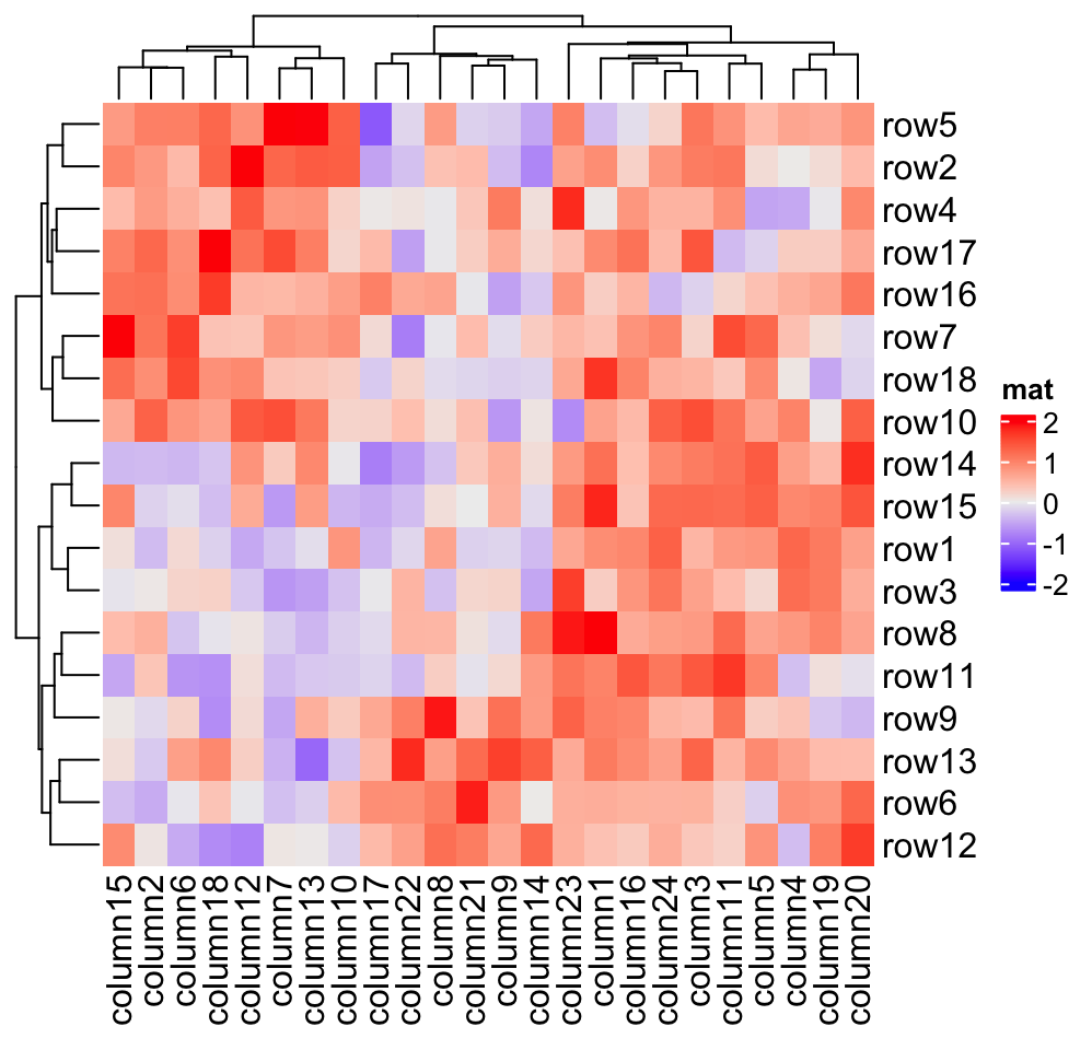
For more use of the seriate() function, please refer to the seriation
package.
2.6 Dimension labels
The row names and column names are drawn on the right and bottom sides of the heatmap by default. Side, visibility and graphics parameters for dimension names can be set as follows:
Heatmap(mat, name = "mat", row_names_side = "left", row_dend_side = "right",
    column_names_side = "top", column_dend_side = "bottom")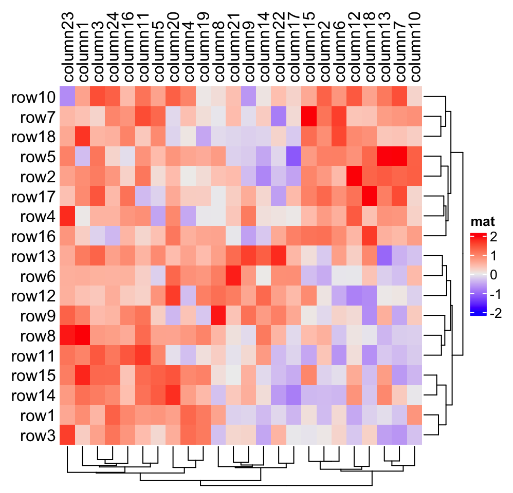
Heatmap(mat, name = "mat", show_row_names = FALSE)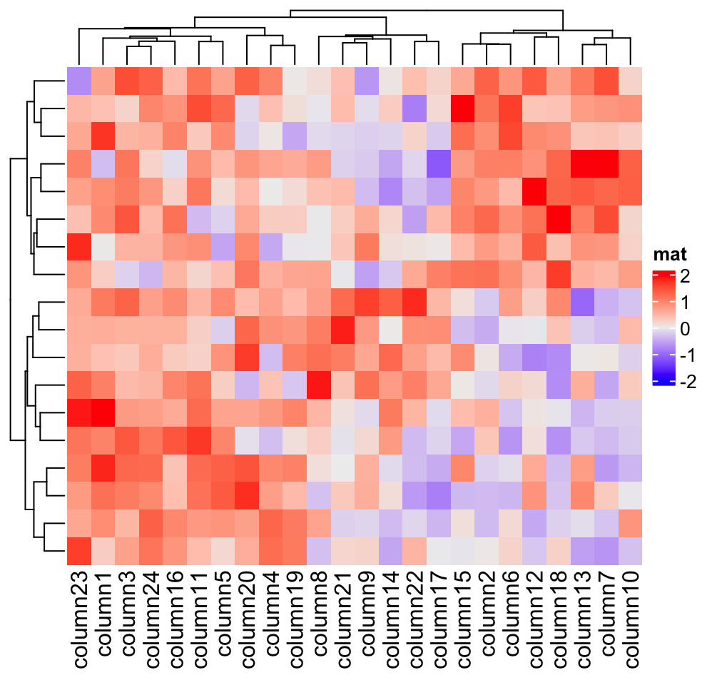
Heatmap(mat, name = "mat", row_names_gp = gpar(fontsize = 20))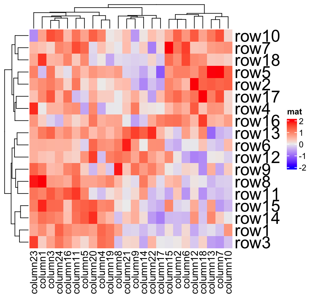

Heatmap(mat, name = "mat",
    row_names_centered = TRUE, column_names_centered = TRUE)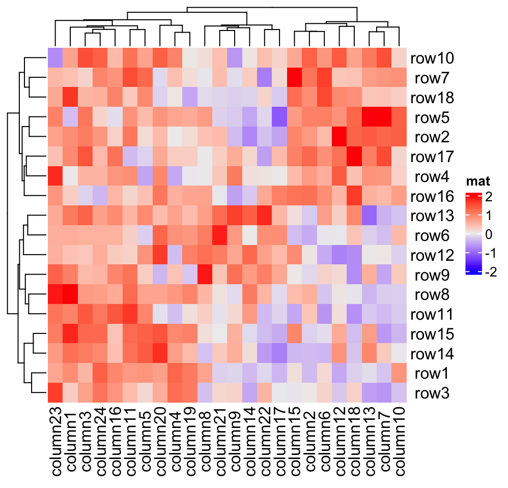
The rotation of column names can be set by column_names_rot:
Heatmap(mat, name = "mat", column_names_rot = 45)
Heatmap(mat, name = "mat", column_names_rot = 45, column_names_side = "top",
    column_dend_side = "bottom")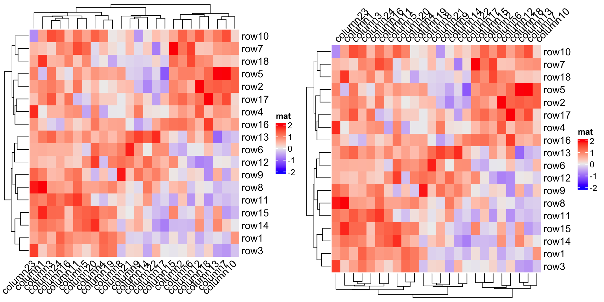
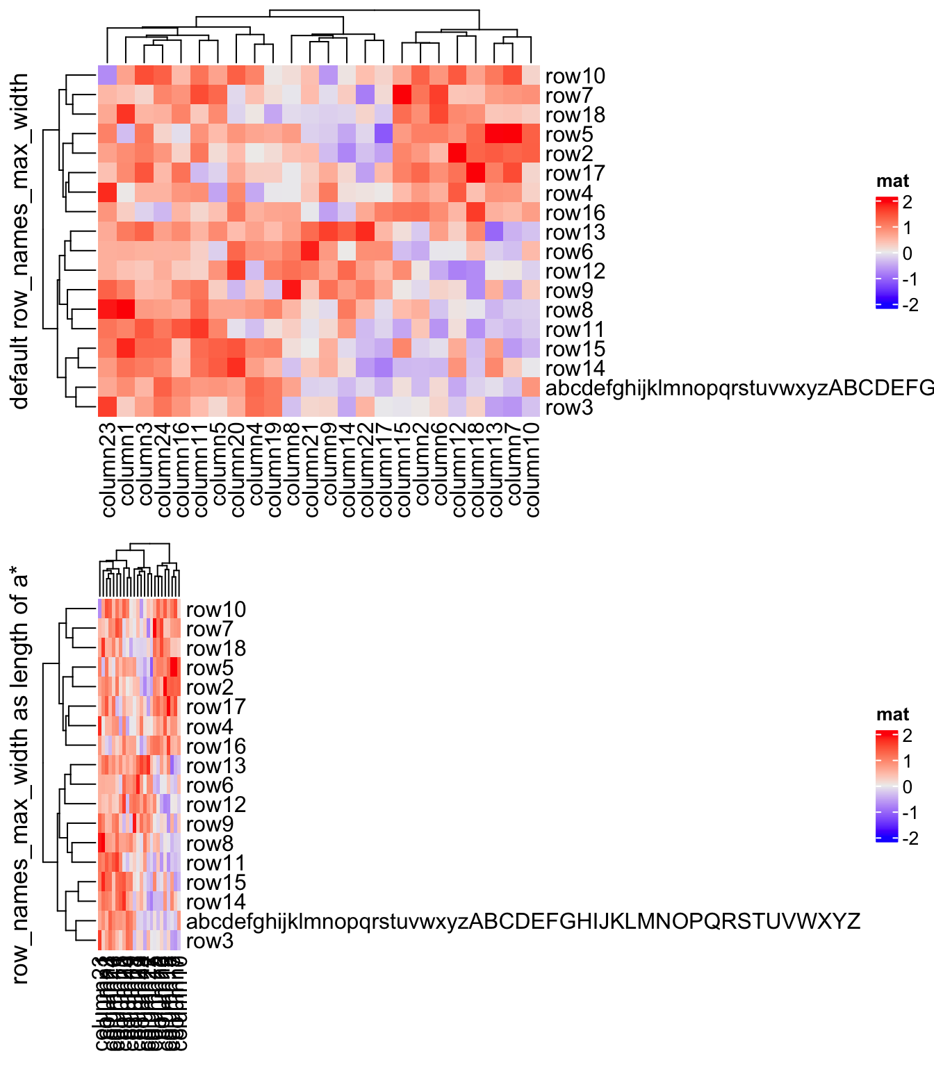
If you have row names or column names which are too long,
row_names_max_width or column_names_max_height can be used to set the
maximal space for them. The default maximal space for row names and column
names are all 6 cm. In following code, max_text_width() is a helper function
to quick calculate maximal width from a vector of text.
mat2 = mat
rownames(mat2)[1] = paste(c(letters, LETTERS), collapse = "")
Heatmap(mat2, name = "mat", row_title = "default row_names_max_width")
Heatmap(mat2, name = "mat", row_title = "row_names_max_width as length of a*",
    row_names_max_width = max_text_width(
        rownames(mat2),
        gp = gpar(fontsize = 12)
    ))
Instead of directly using the row/column names from the matrix, you can also
provide another character vector which corresponds to the rows or columns and
set it by row_labels or column_labels. This is useful because you don’t
need to change the dimension names of the matrix to change the labels on the
heatmap while you can directly provide the new labels.
There is one typical scenario that row_labels and column_labels are
useful. For the gene expression analysis, we might use Ensembl ID as the gene
ID which is used as row names of the gene expression matrix. However, the
Ensembl ID is for the indexing of the Ensembl database but not for the human
reading. Instead, we would prefer to put gene symbols on the heatmap as the
row names which is easier to read. To do this, we only need to assign the
corresponding gene symbols to row_labels without modifying the original
matrix.
The second advantage is row_labels or column_labels allows duplicated
labels, while duplicated row names or column names are not allowed in the
matrix.
Following gives a simple example that we put letters as row labels and column labels:
# use a named vector to make sure the correspondance between
# row names and row labels is correct
row_labels = structure(paste0(letters[1:24], 1:24), names = paste0("row", 1:24))
column_labels = structure(paste0(LETTERS[1:24], 1:24), names = paste0("column", 1:24))
row_labels
## row1 row2 row3 row4 row5 row6 row7 row8 row9 row10 row11 row12 row13
## "a1" "b2" "c3" "d4" "e5" "f6" "g7" "h8" "i9" "j10" "k11" "l12" "m13"
## row14 row15 row16 row17 row18 row19 row20 row21 row22 row23 row24
## "n14" "o15" "p16" "q17" "r18" "s19" "t20" "u21" "v22" "w23" "x24"
Heatmap(mat, name = "mat", row_labels = row_labels[rownames(mat)],
    column_labels = column_labels[colnames(mat)])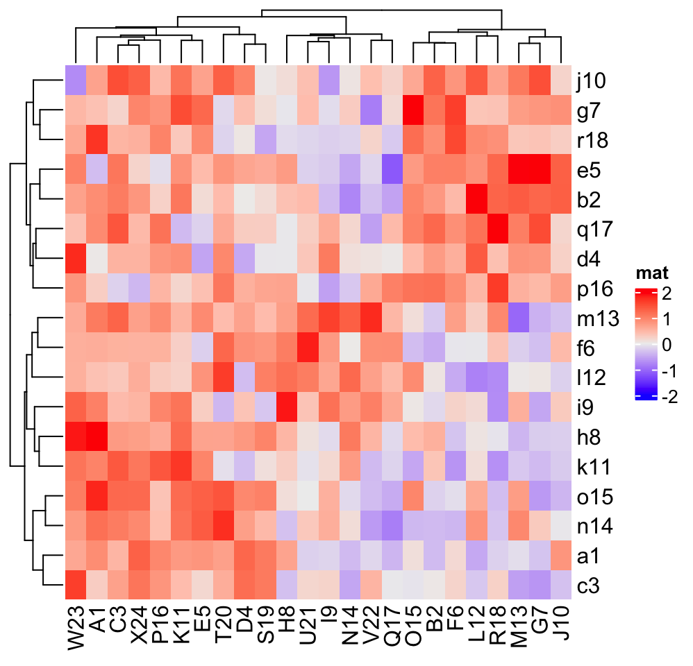
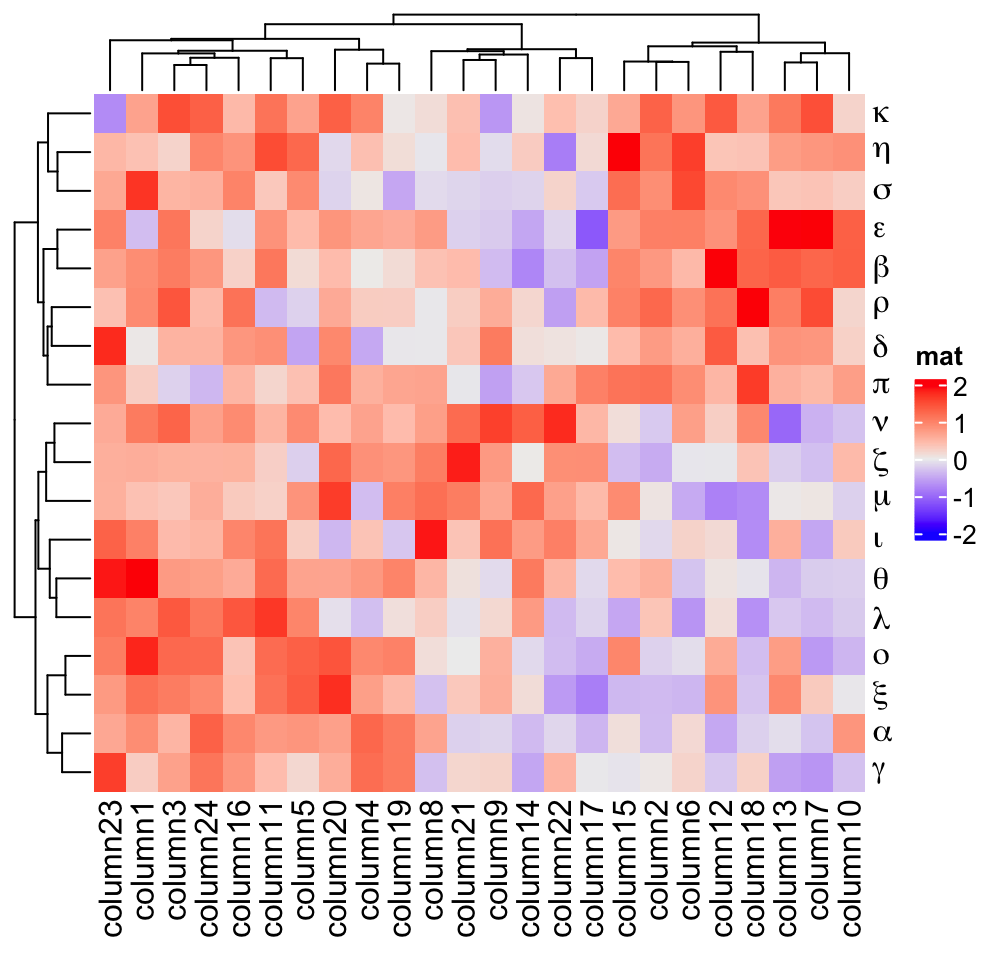
The third advantage is mathematical expression can be used as row names in the heatmap.
Heatmap(mat, name = "mat", row_labels = expression(alpha, beta, gamma,
    delta, epsilon, zeta, eta, theta, iota, kappa, lambda, mu, nu, xi,
    omicron, pi, rho, sigma)
)
The fourth advantage is that you can construct complicated labels with gridtext package. The following is a quick example. More examples can be found in Section 10.3.1.
Heatmap(mat, name = "mat",
    row_labels = gt_render(letters[1:18], padding = unit(c(2, 10, 2, 10), "pt")),
    row_names_gp = gpar(box_col = rep(c("red", "green"), times = 9)))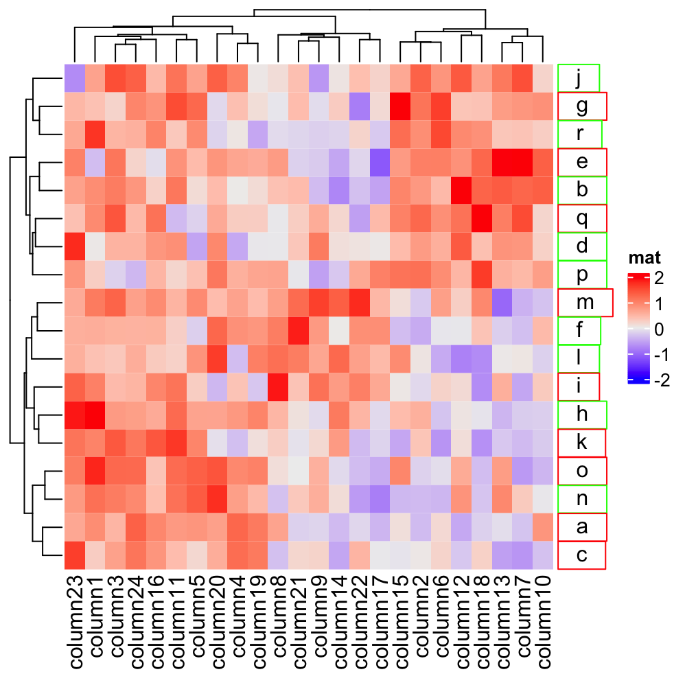
Internally, row names and columns names are actually implemented by the
anno_text() function (Section 3.14), in other words, they
are treated as special cases for text annotations.
2.7 Heatmap split
One major advantage of ComplexHeatmap package is that it supports splitting the heatmap by rows and columns to better group the features and additionally highlight the patterns.
Following arguments control the splitting: row_km, row_split, column_km,
column_split. In following, we call the sub-clusters generated by splitting as
“slices.”
2.7.1 Split by k-means clustering
row_km and column_km apply k-means partitioning.
Heatmap(mat, name = "mat", row_km = 2)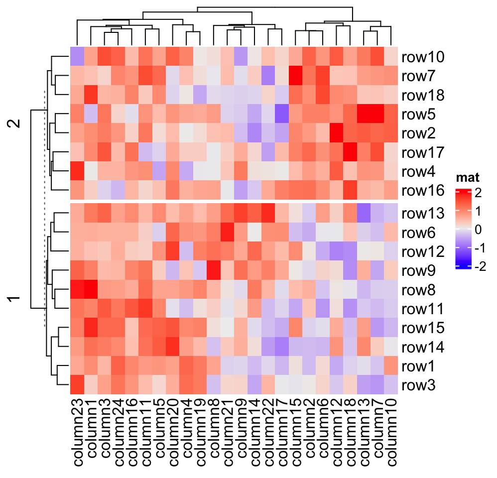
Heatmap(mat, name = "mat", column_km = 3)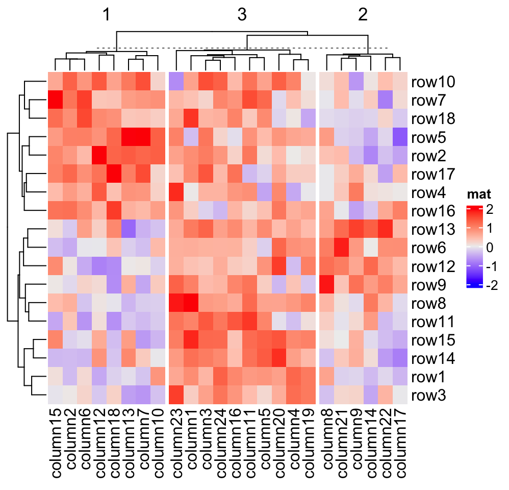
Row splitting and column splitting can be performed simultaneously.
Heatmap(mat, name = "mat", row_km = 2, column_km = 3)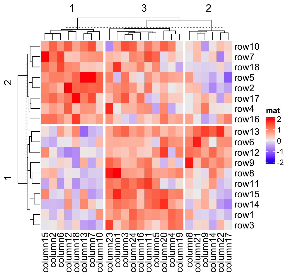
You might notice there are dashed lines in the row and column dendrograms, it will be explained in Section 2.7.2 (the last paragraph).
Heatmap() internally calls kmeans() with random start points, which
results in, for some cases, generating different clusters from repeated runs.
To get rid of this problem, row_km_repeats and column_km_repeats can be
set to a number larger than 1 to run kmeans() multiple times and a final
consensus k-means clustering is used. Please note the final number of clusters
form consensus k-means might be smaller than the number set in row_km and
column_km.
# of course, it will be a little bit slower
Heatmap(mat, name = "mat",
    row_km = 2, row_km_repeats = 100,
    column_km = 3, column_km_repeats = 100)
Note if you want the k-means clustering completely reproducible, you must explicitly set the same random seed:
set.seed(123)
Heatmap(..., row_km = ..., column_km = ...)
2.7.2 Split by categorical variables
More generally, row_split or column_split can be set to a categorical
vector or a data frame where different combinations of levels split the
rows/columns in the heatmap. How to control the order of the slices is
introduced in Section 2.7.4.
# split by a vector
Heatmap(mat, name = "mat",
    row_split = rep(c("A", "B"), 9), column_split = rep(c("C", "D"), 12))
# split by a data frame
Heatmap(mat, name = "mat",
    row_split = data.frame(rep(c("A", "B"), 9), rep(c("C", "D"), each = 9)))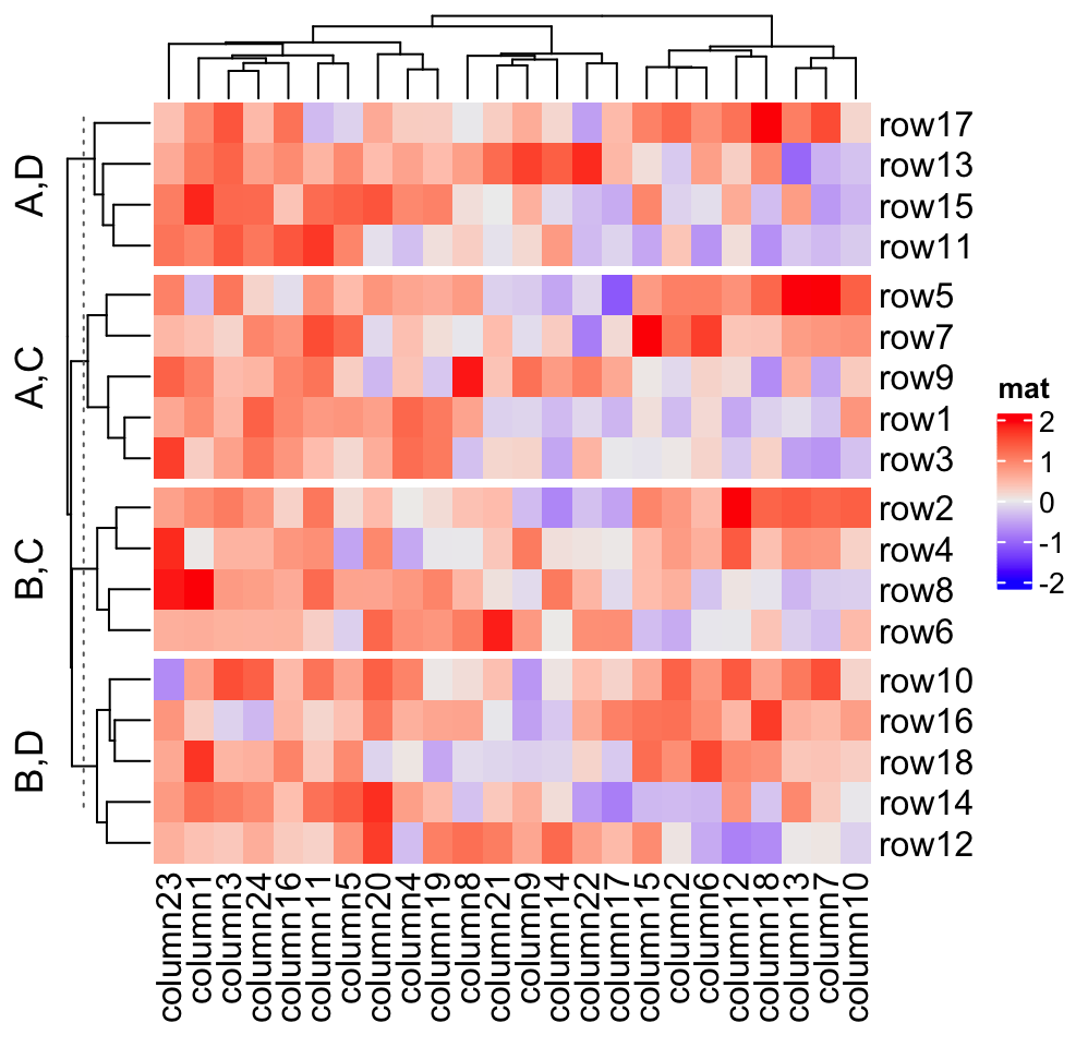
# split on both dimensions
Heatmap(mat, name = "mat", row_split = factor(rep(c("A", "B"), 9)),
    column_split = factor(rep(c("C", "D"), 12)))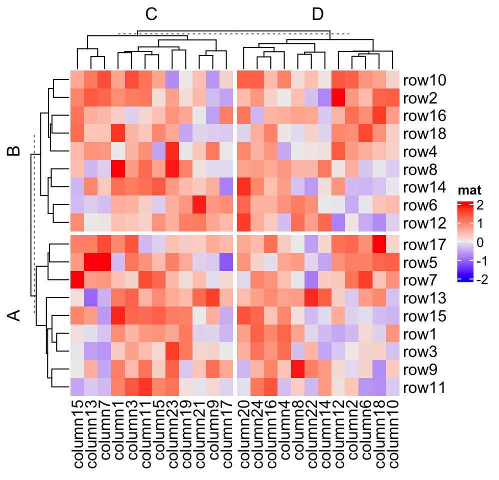
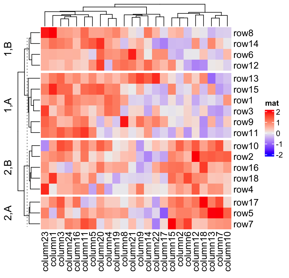
Actually, k-means clustering just generates a vector of cluster classes and
appends to row_split or column_split. row_km/column_km can be used
mixed with row_split and column_split.
which is the same as:
# code only for demonstration
cl = kmeans(mat, centers = 2)$cluster
# classes from k-means are always put as the first column in `row_split`
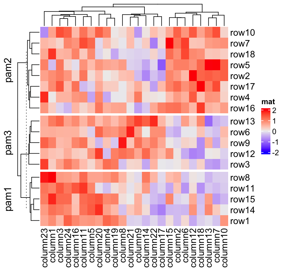
Heatmap(mat, name = "mat", row_split = cbind(cl, rep(c("A", "B"), 9)))If you are not happy with the default k-means partition, it is easy to use
other partition methods by just assigning the partition vector to
row_split/column_split.
If row_order or column_order is set, in each row/column slice, it is still
ordered.
# remember when `row_order` is set, row clustering is turned off
Heatmap(mat, name = "mat", row_order = 18:1, row_km = 2)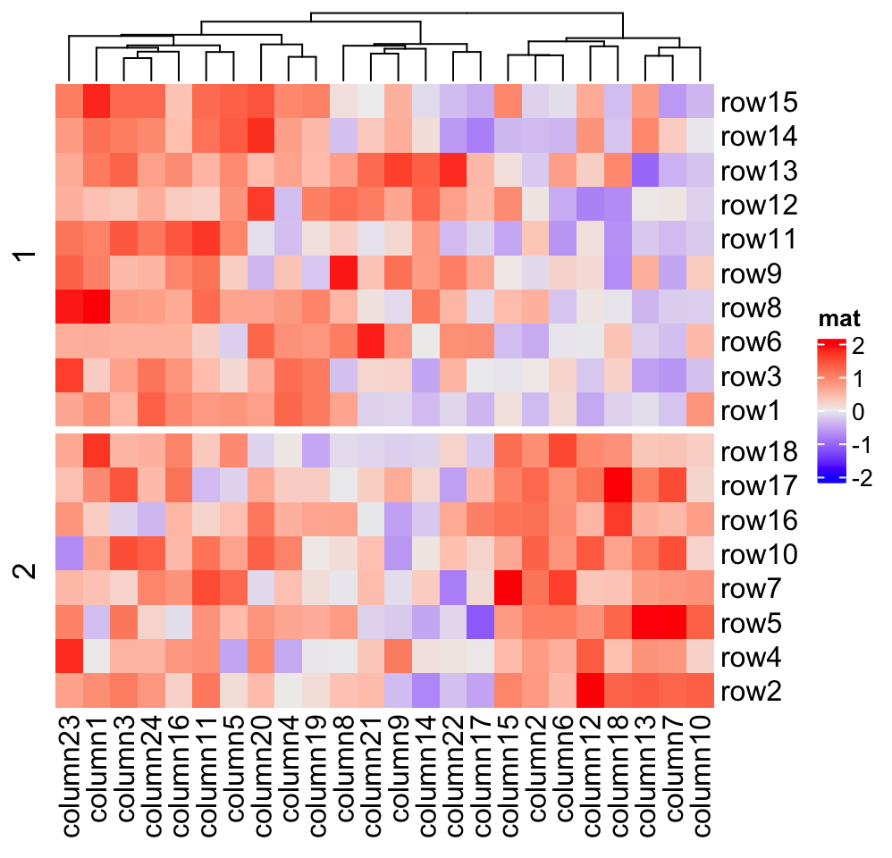
Character matrix can only be split by row_split/column_split argument.
# split by the first column in `discrete_mat`
Heatmap(discrete_mat, name = "mat", col = 1:4, row_split = discrete_mat[, 1])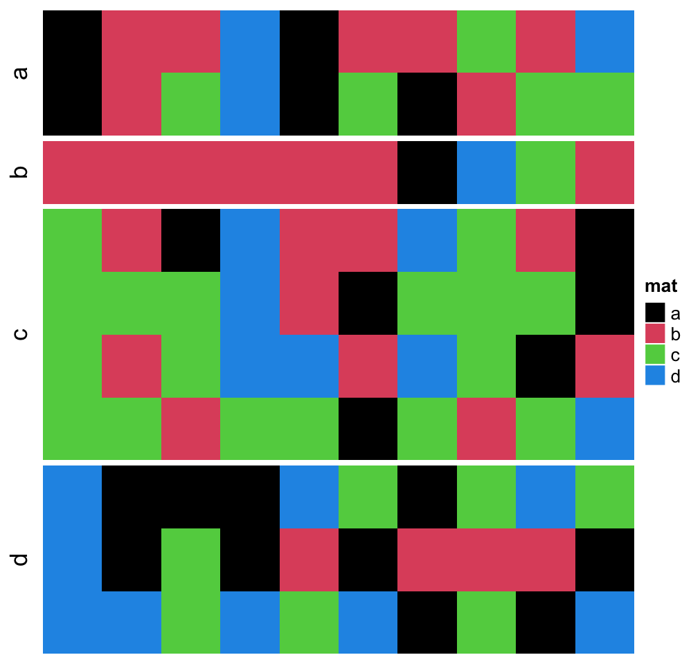
If row_km/column_km is set or row_split/column_split is set as a
vector or a data frame, hierarchical clustering is first applied to each slice
which generates k dendrograms, then a parent dendrogram is generated based
on the mean values of each slice. The height of the parent dendrogram is
adjusted by adding the maximal height of the dendrograms in all child
slices and the parent dendrogram is added on top of the child dendrograms
to form a single global dendrogram. This is why you see dashed lines in the
dendrograms in previous heatmaps. They are used to discriminate the parent dendrogram
and the child dendrograms, and alert users they are calculated in different
ways. These dashed lines can be removed by setting show_parent_dend_line = FALSE in Heatmap(), or set it as a global option:
ht_opt$show_parent_dend_line = FALSE, but we are not suggested to do so.
Heatmap(mat, name = "mat", row_km = 2, column_km = 3,
    show_parent_dend_line = FALSE)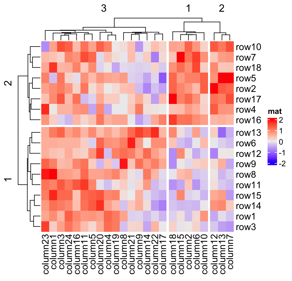
2.7.3 Split by dendrogram
A second scenario for splitting is that users may still want to keep the
global dendrogram which is generated from the complete matrix. In this case, row_split/column_split can be
set to a single number which will apply cutree() on the row/column
dendrogram. This works when cluster_rows/cluster_columns is set to TRUE
or is assigned with a hclust/dendrogram object.
For this case, the dendrogram is still as same as the original one, except that the positions of dendrogram leaves are slightly adjusted by the gaps between slices. (There is no dashed lines, because here the dendrogram is calcualted as a complete one and there is no parent dendrogram or child dendrograms.)
Heatmap(mat, name = "mat", row_split = 2, column_split = 3)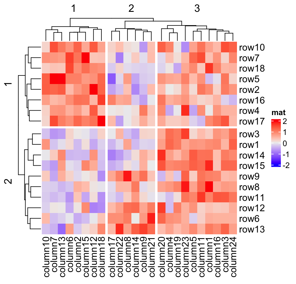
dend = as.dendrogram(hclust(dist(mat)))
dend = color_branches(dend, k = 2)
Heatmap(mat, name = "mat", cluster_rows = dend, row_split = 2)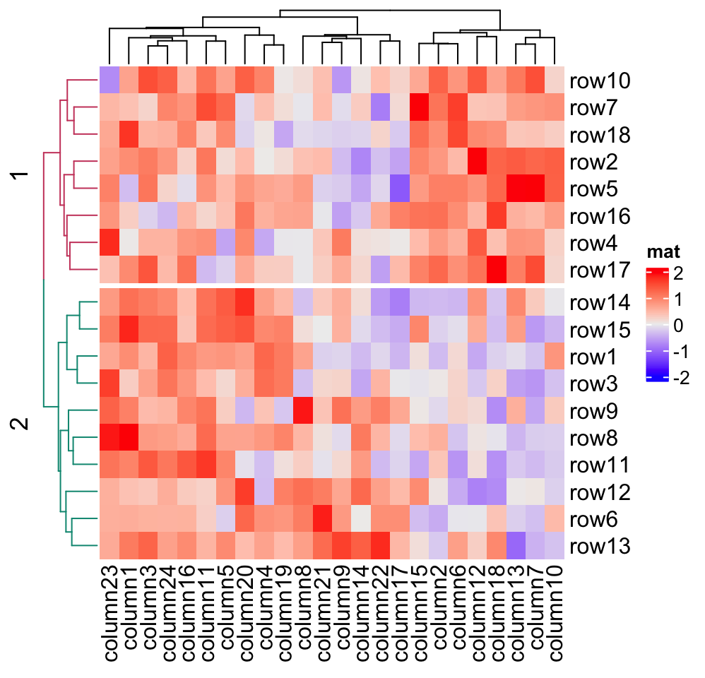
If you want to combine splitting from cutree() and other categorical
variables, you need to generate the partitions from cutree() in the first
place, append to e.g. row_split as a data frame and then send it to
row_split argument.
2.7.4 Order of slices
When row_split/column_split is set as a categorical variable (a vector or a
data frame) or row_km/column_km is set, by default, there is an additional
clustering applied to the mean of slices to show the hierarchy on the slice
level. Under this scenario, you cannot precisely control the order of slices
because it is controlled by the clustering of slices.
Nevertheless, you can set cluster_row_slices or cluster_column_slices to
FALSE to turn off the clustering on slices, and now you can precisely
control the order of slices.
When there is no slice clustering, the order of each slice can be controlled
by levels of each variable in row_split/column_split (in this case, each
variable should be a factor). If all variables are characters, the default
order is unique(row_split) or unique(column_split). Compare following
heatmaps:
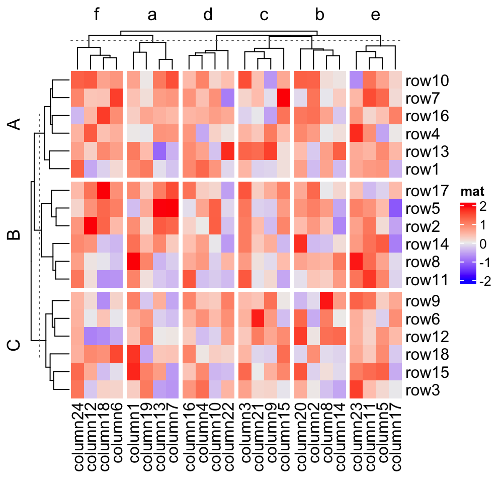
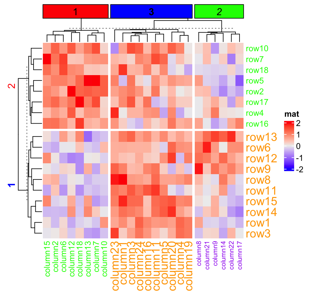
# clustering is similar as previous heatmap with branches
# in some nodes in the dendrogram flipped
Heatmap(mat, name = "mat",
    row_split = factor(rep(LETTERS[1:3], 6), levels = LETTERS[3:1]),
    column_split = factor(rep(letters[1:6], 4), levels = letters[6:1]))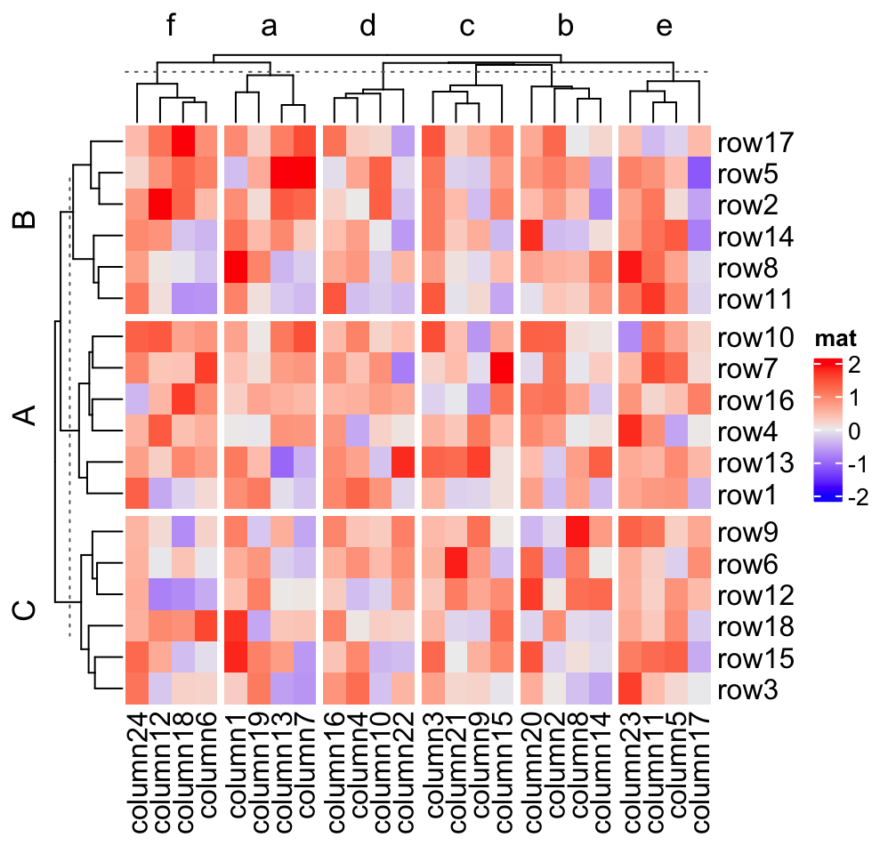
# now the order is exactly what we set
Heatmap(mat, name = "mat",
    row_split = factor(rep(LETTERS[1:3], 6), levels = LETTERS[3:1]),
    column_split = factor(rep(letters[1:6], 4), levels = letters[6:1]),
    cluster_row_slices = FALSE,
    cluster_column_slices = FALSE)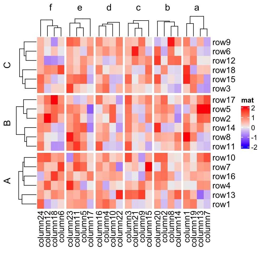
Also you can see in the third heatmap, when cluster_row_slices and cluster_column_slices
are set to FALSE, there is no dendrogram on slice level.
2.7.5 Titles for splitting
When row_split/column_split is set as a single number, there is only one
categorical variable, while when row_km/column_km is set and/or
row_split/column_split is set as categorical variables, there will be
multiple categorical variables. By default, the titles are in a form of
"level1,level2,..." which corresponds to every combination of levels in all
categorical variables. The titles for splitting can be controlled by “a
template.”
ComplexHeatmap supports three types of templates. The first one is by
sprintf() where the %s is replaced by the corresponding level. In
following example, since all combinations of split are c("A", "C"), c("A", "D"), c("B", "C")
and c("B", "D"), if row_title is set to %s|%s, the four row titles will be
A|C, A|D, B|C, B|D.
split = data.frame(rep(c("A", "B"), 9), rep(c("C", "D"), each = 9))
Heatmap(mat, name = "mat", row_split = split, row_title = "%s|%s")
For the sprintf() template, you can only put the levels which are A,B,C,D
in the title, and C,D is always after A,B (i.e. it always A,C and
A,D). However, when making the heatmap, you might want to put more
meaningful text instead of the internal levels. Once you know how to
correspond the text to the level, you can add it by the following two other template
methods.
In the following two template methods, special marks are used to mark the R
code which is executable (it is called variable interpolation where the code
is extracted and executed and the returned value in put back to the string).
There are two types of template marks @{} and {}. The first one is from
GetoptLong package which should already be installed when you install the
ComplexHeatmap package and the second one is from glue package which
you need to install first.
There is an internal variable x you should use when you use the latter two
templates. x is just a simple vector which contains current category levels
(e.g. c("A", "C")).
# We only run the code for the first heatmap
map = c("A" = "aaa", "B" = "bbb", "C" = "333", "D" = "444")
Heatmap(mat, name = "mat", row_split = split,
    row_title = "@{map[ x[1] ]}|@{map[ x[2] ]}")
Heatmap(mat, name = "mat", row_split = split,
    row_title = "{map[ x[1] ]}|{map[ x[2] ]}")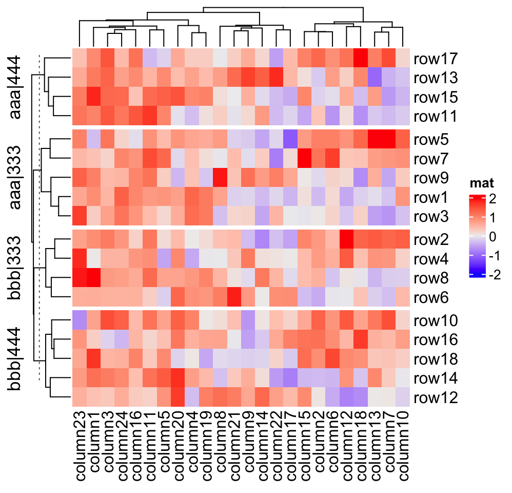
The row title is rotated by default, you can set row_title_rot = 0 to make
it horizontal:
Heatmap(mat, name = "mat", row_split = split, row_title = "%s|%s",
    row_title_rot = 0)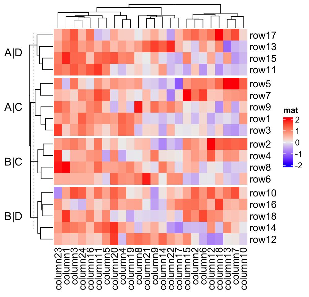
When row_split/column_split is set as a number, you can also use template
to adjust the titles for slices.
Heatmap(mat, name = "mat", row_split = 2, row_title = "cluster_%s")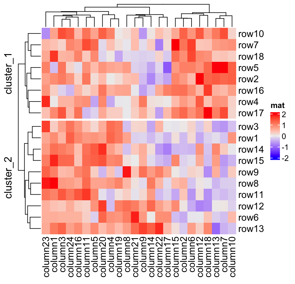
If you know the final number of row slices, you can directly set a vector of
titles to row_title. Be careful the number of row slices is not always
identical to n_level_1 * n_level_2 * ....
# we know there are four slices
Heatmap(mat, name = "mat", row_split = split,
    row_title = c("top_slice", "middle_top_slice", "middle_bottom_slice", "bottom_slice"),
    row_title_rot = 0)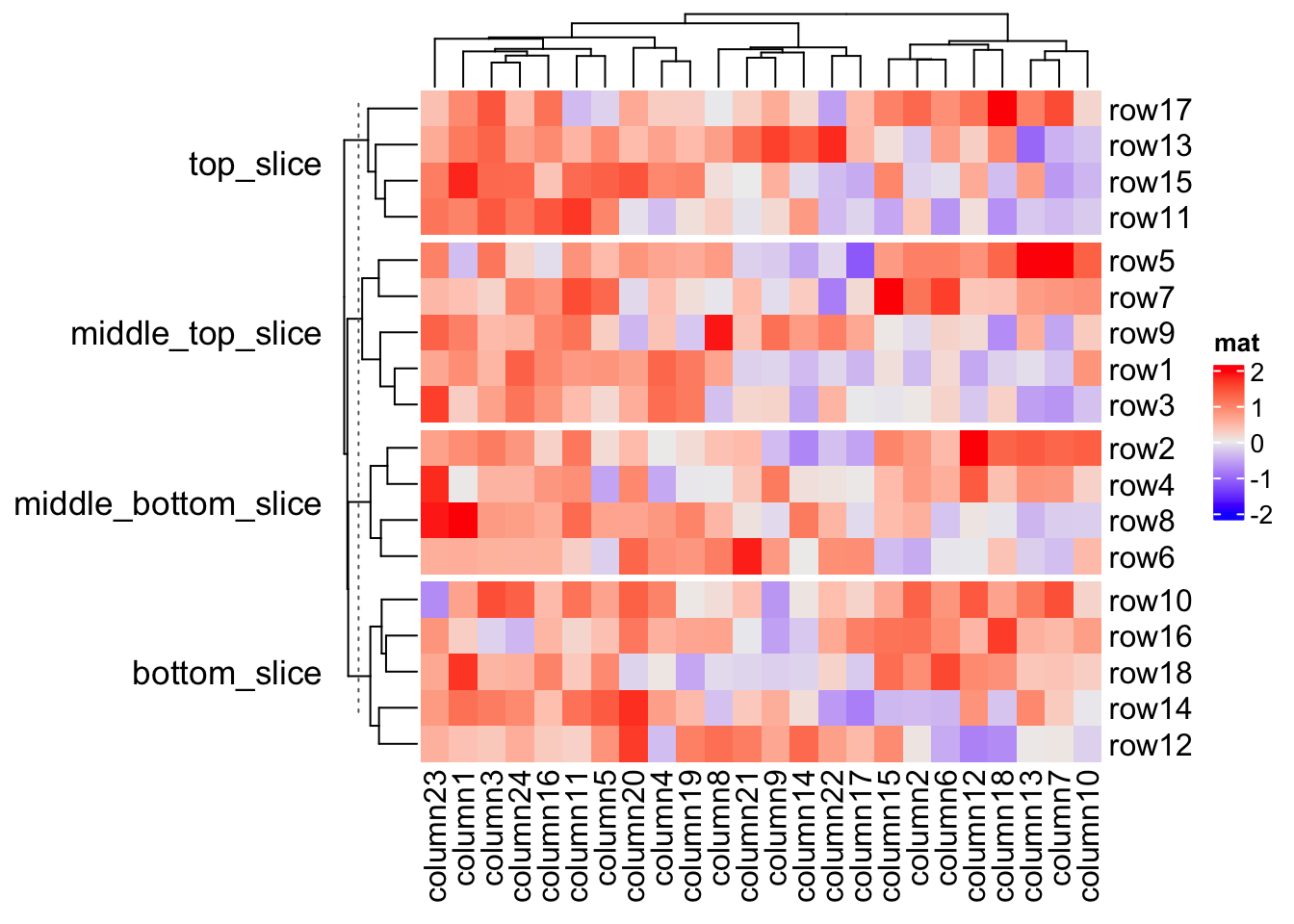
If the length of row_title is specified as a single string, it will be like
a single title for all slices.
Heatmap(mat, name = "mat", row_split = split, row_title = "there are four slices")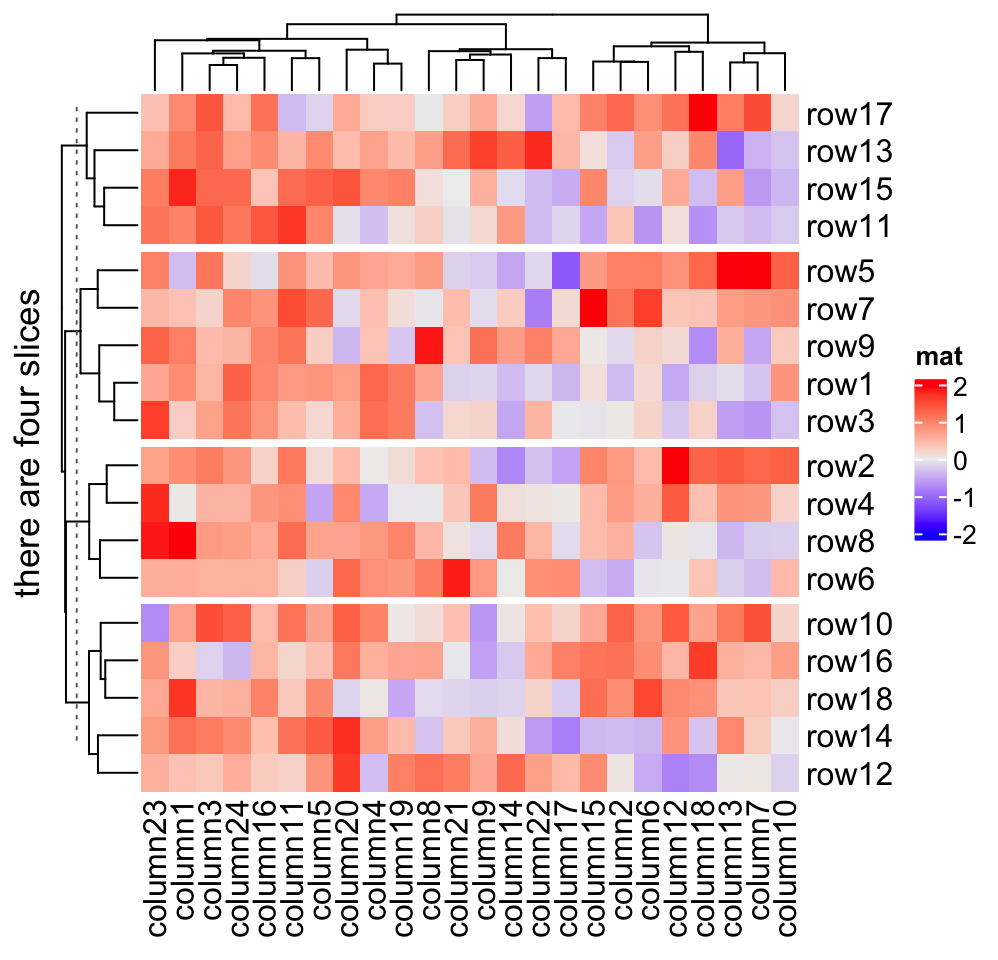
If you still want titles for each slice, but also a global title, you can do as follows.
ht = Heatmap(mat, name = "mat", row_split = split, row_title = "%s|%s")
# This row_title is actually a heatmap-list-level row title
draw(ht, row_title = "I am a row title")
Actually the row_title used in draw() function is the row title of the
heatmap list (although in the example there is only one heatmap). The draw()
function and the heatmap list will be introduced in Chapter
4.
If row_title is set to NULL, no row title is drawn.
Heatmap(mat, name = "mat", row_split = split, row_title = NULL)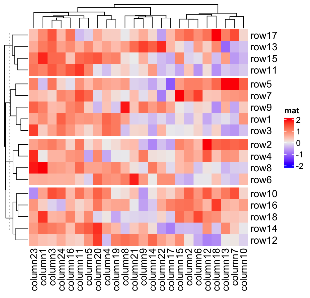
All these rules also work for column titles for slices.
2.7.6 Graphic parameters for splitting
When splitting is applied on rows/columns, graphic parameters for row/column title and row/column names can be specified as same length as number of slices.
# by defalt, there no space on the top of the title, here we add 4pt to the top.
# it can be reset by `ht_opt(RESET = TRUE)`
ht_opt$TITLE_PADDING = unit(c(4, 4), "points")
Heatmap(mat, name = "mat",
    row_km = 2,
    row_title_gp = gpar(col = c("red", "blue"), font = 1:2),
    row_names_gp = gpar(col = c("green", "orange"), fontsize = c(10, 14)),
    column_km = 3,
    column_title_gp = gpar(fill = c("red", "blue", "green"), font = 1:3),
    column_names_gp = gpar(col = c("green", "orange", "purple"),
        fontsize = c(10, 14, 8))
)
2.7.7 Gaps between slices
The space of gaps between row/column slices can be controlled by
row_gap/column_gap. The value can be a single unit or a vector of units.
Heatmap(mat, name = "mat", row_km = 3, row_gap = unit(5, "mm"))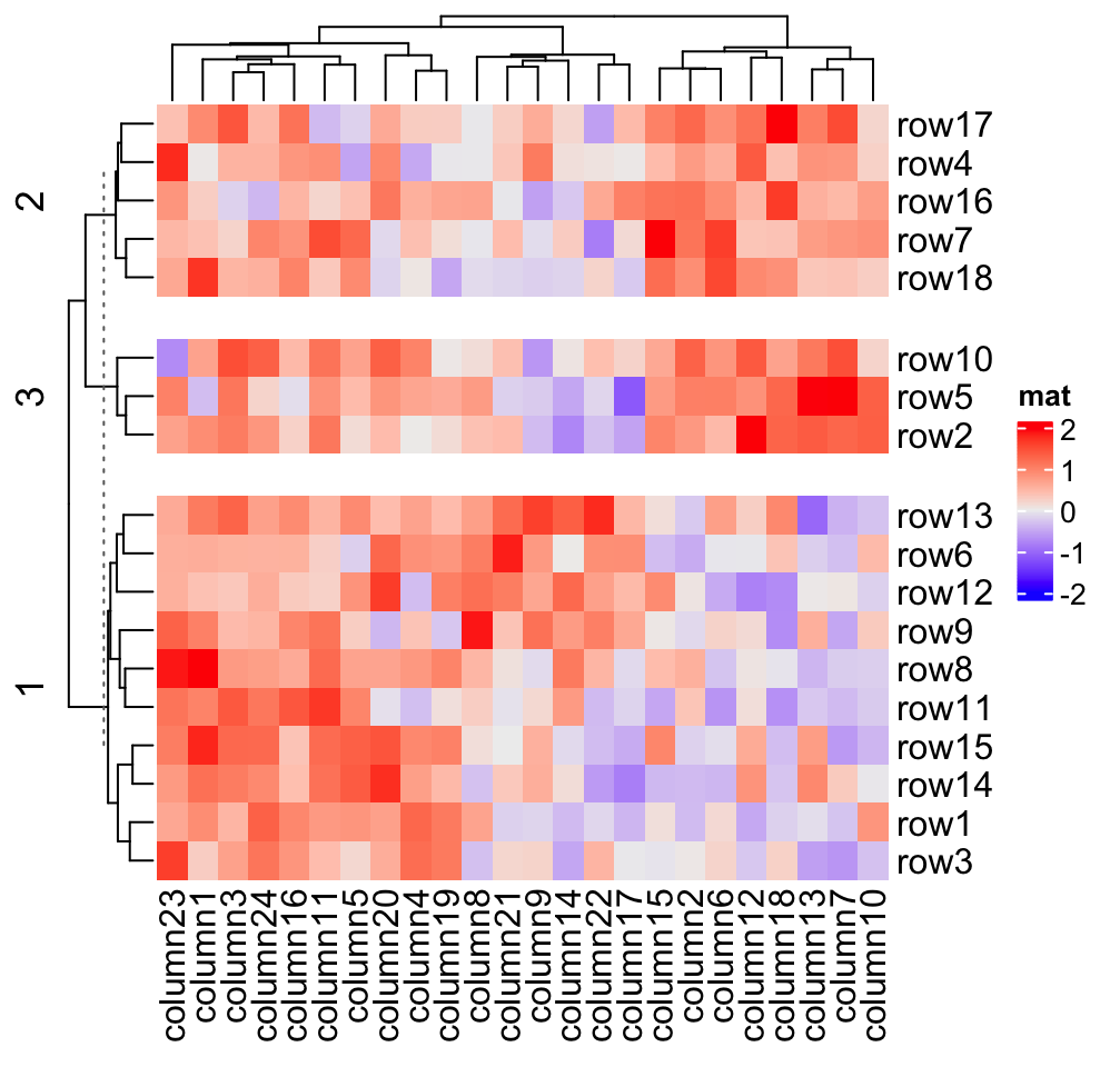
Heatmap(mat, name = "mat", row_km = 3, row_gap = unit(c(2, 4), "mm"))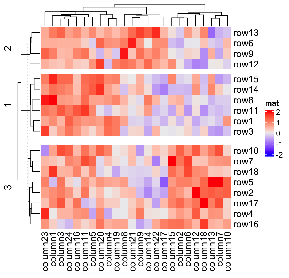
Heatmap(mat, name = "mat", row_km = 3, row_gap = unit(c(2, 4), "mm"),
    column_km = 3, column_gap = unit(c(2, 4), "mm"))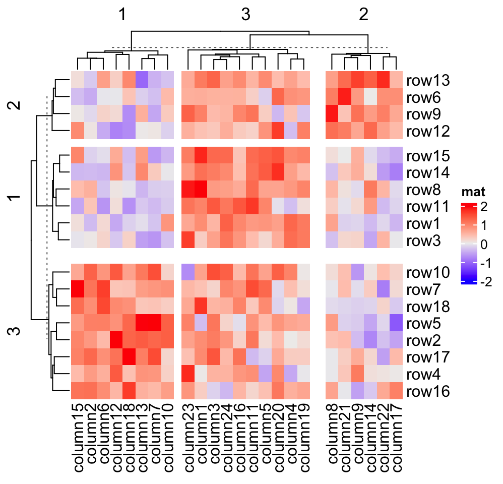
When heatmap border is added by setting border = TRUE, the border of every
slice is added.
Heatmap(mat, name = "mat", row_km = 2, column_km = 3, border = TRUE)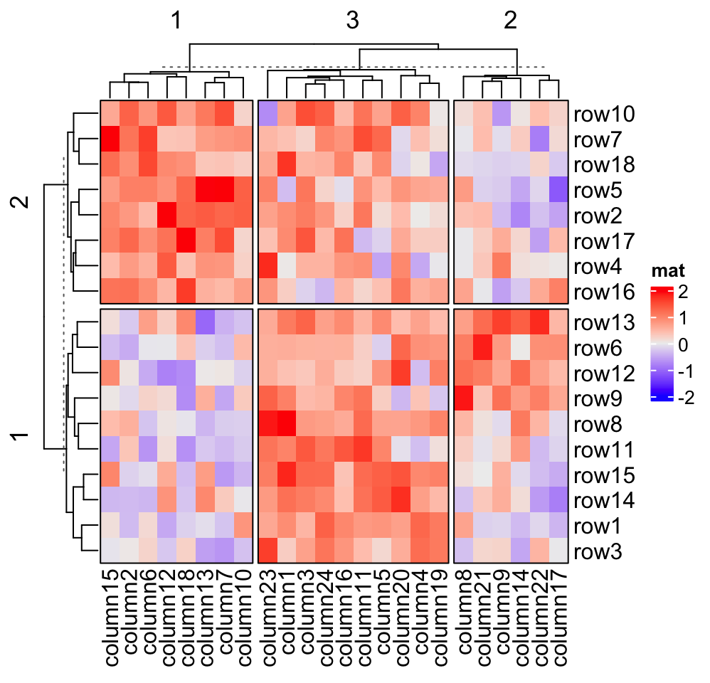
If you set gap size to zero, the heatmap will look like it is partitioned by vertical and horizontal lines.
Heatmap(mat, name = "mat", row_km = 2, column_km = 3,
    row_gap = unit(0, "mm"), column_gap = unit(0, "mm"), border = TRUE)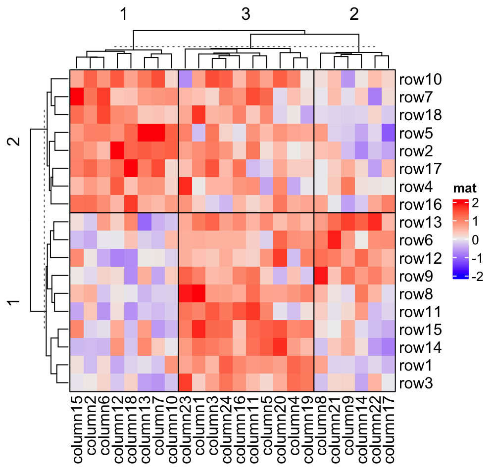
2.7.8 Split heatmap annotations
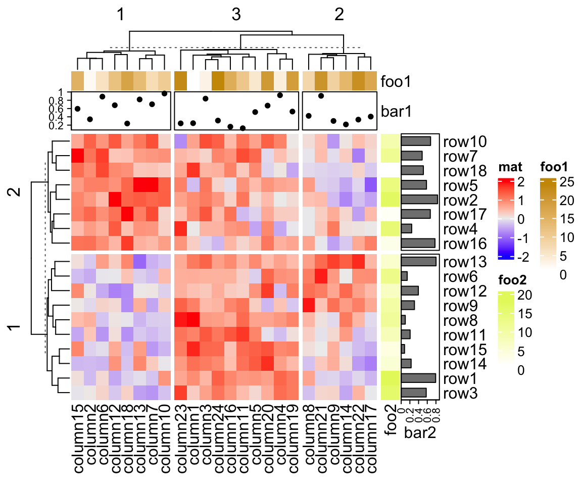
When the heatmap is split, all the heatmap components are split accordingly. Following gives you a simple example and the heatmap annotation will be introduced in Chapter 3.
Heatmap(mat, name = "mat", row_km = 2, column_km = 3,
    top_annotation = HeatmapAnnotation(foo1 = 1:24, bar1 = anno_points(runif(24))),
    right_annotation = rowAnnotation(foo2 = 18:1, bar2 = anno_barplot(runif(18)))
)
2.8 Heatmap as raster image
When we produce so-called “high quality figures,” normally we save the figures as vector graphics in the format of e.g. pdf or svg. The vector graphics basically store details of every single graphic elements, thus, if a heatmap made from a very huge matrix is saved as vector graphics, the final file size would be very big. On the other hand, when visualizing e.g. the pdf file on the screen, multiple grids from the heatmap actually only map to single pixels, due to the limited size of the screen. Thus, there need some ways to effectively reduce the original image and it is not necessary to store the complete matrix for the heatmap.
Rasterization is a way to covnert the vector graphics into a matrix of colors. In this case, an image is represented as a matrix of RGB values, which is called a raster image. If the heatmap is larger than the size of the screen or the pixels that current graphics devices can support, we can convert the heatmap and reduce it, by saving it in a form of a color matrix with the same dimension as on the device.
Let’s assume a matrix has \(n_r\) rows and \(n_c\) columns. When it is drawn on a certain graphics device, e.g. an on-screen device, the corresponding heatmap body has \(p_r\) and \(p_c\) pixels (or points) for the rows and columns, respectively. When \(n_r > p_r\) and/or \(n_c > p_c\), multiple values in the matrix are mapped to single pixels. Here we need to reduce \(n_r\) and/or \(n_c\) if they are larger than \(p_r\) and/or \(p_c\).
To make it simple, I assume both \(n_r > p_r\) and \(n_c > p_c\). The principle is basically the same for the scenarios where only one dimension of the matrix is larger than the device.
From ComplexHeatmap version 2.5.4, there are following three implementations for image rasterization. Note the implementation is a little bit different from the earlier versions (of course, better than the earlier versions).
-
First an image (in a specific format, e.g. png or jpeg) with \((p_r \cdot a) \times (p_c \cdot a)\) resolution is saved into a temporary file (e.g., by
png()orjpeg()) where \(a\) is a zooming factor, next it is read back as arasterobject by e.g.png::readPNG()orjpeg::readJPEG(), and later the raster object is filled into the heatmap body bygrid::grid.raster(). So we can say, the rasterization is done by the raster image devices (png()orjpeg()).This type of rasterization is automatically turned on (if magick package is not installed) when the number of rows or columns exceeds 2000 (You will see a message. It won’t happen silently). It can also be manually controlled by setting the
use_rasterargument:
Heatmap(..., use_raster = TRUE)The zooming factor is controlled by raster_quality argument. A value larger
than 1 generates files with larger size.
Heatmap(..., use_raster = TRUE, raster_quality = 5)-
Simply reduce the original matrix to \(p_r \times p_c\) where now each single values can correspond to single pixels. In the reduction, a user-defined function is applied to summarize the sub-matrices.
This can be set by
raster_resize_matargument:
# the default summary function is mean()
Heatmap(..., use_raster = TRUE, raster_resize_mat = TRUE)
# use max() as the summary function
Heatmap(..., use_raster = TRUE, raster_resize_mat = max)
# randomly pick one
Heatmap(..., use_raster = TRUE, raster_resize_mat = function(x) sample(x, 1))-
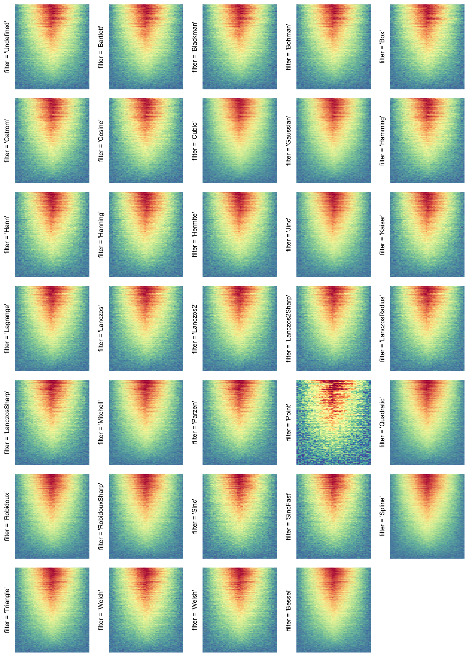
A temporary image with complete resolution \(n_r \times n_c\) is first generated, here
magick::image_resize()is used to reduce the image to size \(p_r \times p_c\). Finally the reduced image is read as arasterobject and filled into the heatmap body. magick provides a lot of methods for “resizing”/“scaling” the image, which is called the “filtering methods” under the term of magick. All filtering methods can be obtained bymagick::filter_types().This type of rasterization can be truned on by setting
raster_by_magick = TRUEand choosing a properraster_magick_filter.
Heatmap(..., use_raster = TRUE, raster_by_magick = TRUE)
Heatmap(..., use_raster = TRUE, raster_by_magick = TRUE, raster_magick_filter = ...)
The type of temporary image is controlled by raster_device argument. All supported
“raster devices” are: png, CairoPNG, agg_png, jpeg, tiff, CairoJPEG and
CairoTIFF. CairoPNG is taken as the default raster device (If Cairo package is installed) because the previously
default device png occasionally produces white vertical and horizontal lines in the
raster image.
In ComplexHeatmap, use_raster is by default turned on if the number of
rows or columns is more than 2000 in the matrix.
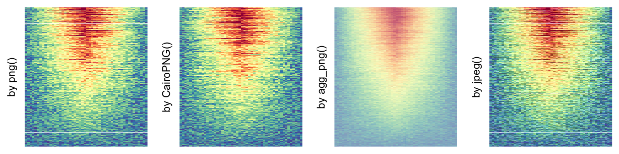
In the following parts of this section, we compare the visual difference between different image rasterization methods. The following example is from Guillaume Devailly’s simulated data but with small adaptations. This example shows an enrichment pattern to the top center of the plot.
In the folowing examples, We won’t show the code for making heatmaps because there are too many heatmaps and the specific settings is already written as the row title of each heatmap. We set the same color mapping for all heatmaps, so that you can see how different rasterizations change the original patterns.
For the comparison, we generated many heatmaps. They can be categoried into three groups, as corresponded to the three rasterization methods mentioned previously.
- by
png()/CairoPNG()/agg_png()/jpeg(): Rasterization method 1. First row in the following heatmaps. -
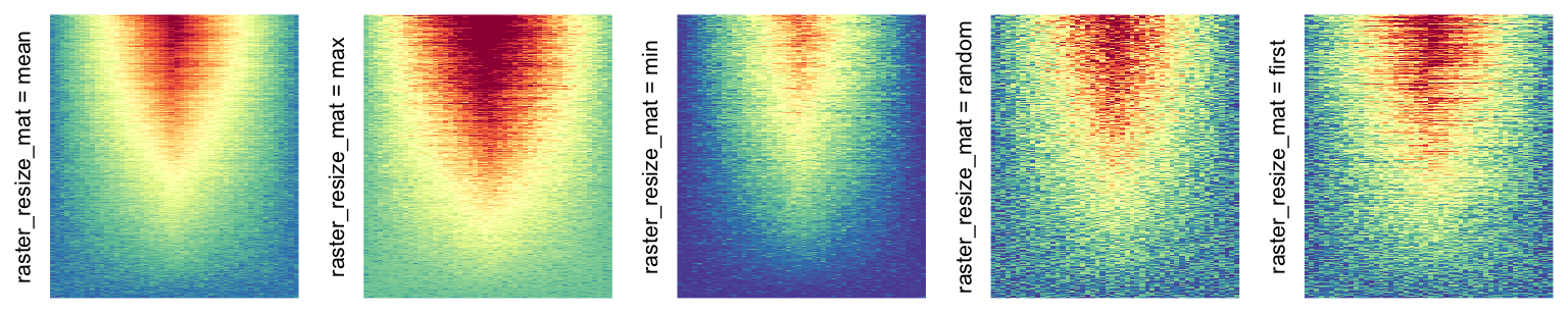
raster_resize_mat = *: Rasterization method 2, with different summary methods. Second row in the following heatmaps. -
filter = *: Rasterization method 3, with different filterring method. The stringfiltershould beraster_magick_filter. It is truncated so that the row title won’t be cut by the plot regions.
More examples on image rasteration can be found in this blog post: Rasterization in ComplexHeatmap.
According to the examples that have been shown, we would say
rasterization by magick package performs better, thus, by default, in
ComplexHeatmap, the rasterization is done by magick (with "Lanczos"
as the default filter method) and if magick is not installed, it uses
CairoPNG() and a friendly message is printed to suggest users to install
magick.
Following example compares the PDF file size with raster images by different raster devices.
library(GetoptLong)
set.seed(123)
mat2 = matrix(rnorm(10000*100), ncol = 100)
pdf(qq("heatmap_no_rasteration.pdf"), width = 8, height = 8)
ht = Heatmap(mat2, cluster_rows = FALSE, cluster_columns = FALSE, use_raster = FALSE)
draw(ht)
dev.off()

all_devices = c("png", "CairoPNG", "agg_png", "jpeg", "CairoJPEG")
for(device in all_devices) {
    pdf(qq("heatmap_@{device}.pdf"), width = 8, height = 8)
    ht = Heatmap(mat2, cluster_rows = FALSE, cluster_columns = FALSE, use_raster = TRUE,
        raster_device = device)
    draw(ht)
    dev.off()
}
all_files = qq("heatmap_@{all_devices}.pdf", collapse = FALSE)
all_files = c("heatmap_no_rasteration.pdf", all_files)
fs = file.size(all_files)
names(fs) = all_files
sapply(fs, function(x) paste(round(x/1024), "KB"))
## heatmap_no_rasteration.pdf heatmap_png.pdf
## "6394 KB" "175 KB"
## heatmap_CairoPNG.pdf heatmap_agg_png.pdf
## "177 KB" "308 KB"
## heatmap_jpeg.pdf heatmap_CairoJPEG.pdf
## "667 KB" "677 KB"We can see png-family methods generate smaller file size.
2.9 Customize the heatmap body
The heatmap body can be self-defined to add more types of graphics. By default
the heatmap body is composed by a matrix of small rectangles (it might be
called grids in other parts of this documentation, but let’s call it “cells”
here) with different filled colors. However, it is also possible to add more
graphics or symbols as additional layers on the heatmap. There are two
arguments cell_fun and layer_fun which both should be user-defined
functions.
In later chapter, we will introduce OncoPrint (Chapter 7), UpSet plot (Chapter 8)
and 3D heatmap (Chapter 12). They are all implemented with cell_fun/layer_fun.
2.9.1 cell_fun
cell_fun draws in each cell repeatedly, which is internally executed in two
nested for loops, while layer_fun is the vectorized version of cell_fun.
cell_fun is easier to understand but layer_fun is much faster to execute
and more customizable.
cell_fun expects a function with 7 arguments (the argument names can be
different from following, but the order must be the same), which are:
-
j: column index in the matrix. Column index corresponds to the x-direction in the viewport, that’s whyjis put as the first argument. -
i: row index in the matrix. -
x: x coordinate of middle point of the cell which is measured in the viewport of the heatmap body. -
y: y coordinate of middle point of the cell which is measured in the viewport of the heatmap body. -
width: width of the cell. The value isunit(1/ncol(sub_mat), "npc")wheresub_matcorrespond to the sub-matrix by row splitting and column splitting. -
height: height of the cell. The value isunit(1/nrow(sub_mat), "npc"). -
fill: color of the cell.
The values for the seven arguments are automatically sent to the function when executed in each cell.
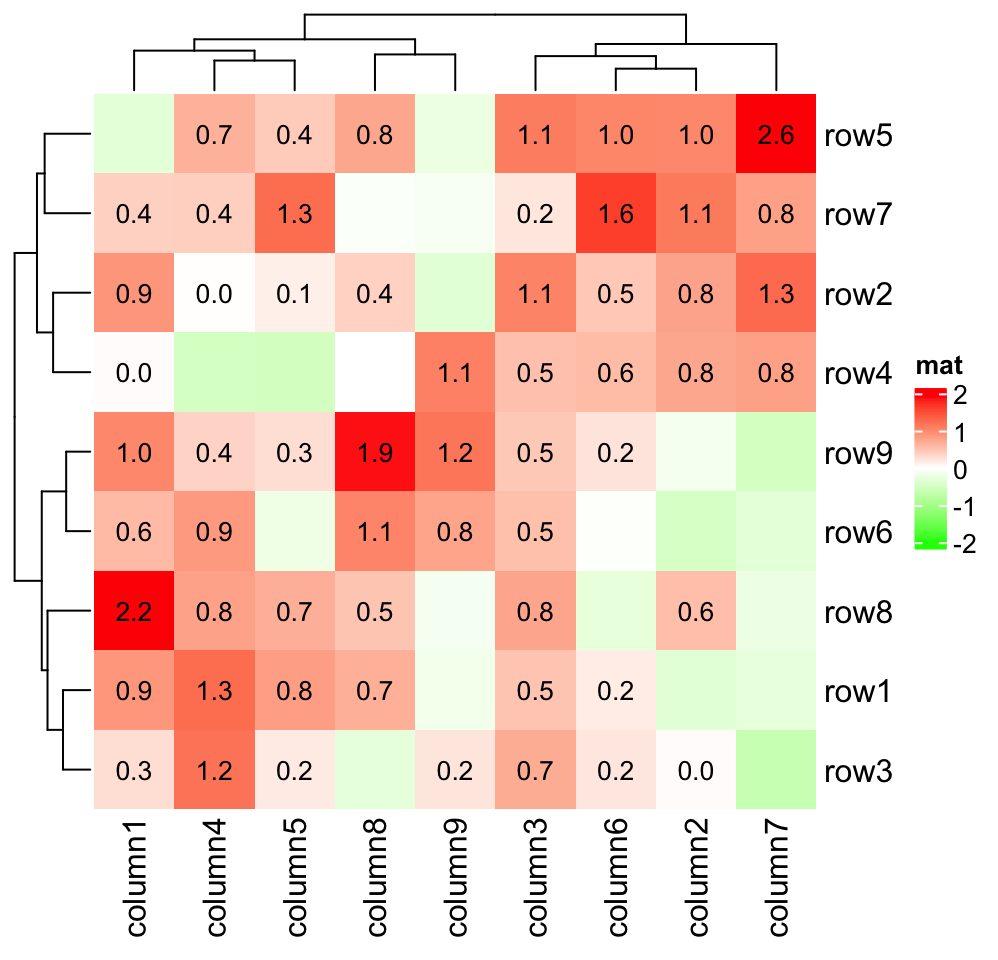
The most common use is to add values in the matrix onto the heatmap:
small_mat = mat[1:9, 1:9]
col_fun = colorRamp2(c(-2, 0, 2), c("green", "white", "red"))
Heatmap(small_mat, name = "mat", col = col_fun,
    cell_fun = function(j, i, x, y, width, height, fill) {
        grid.text(sprintf("%.1f", small_mat[i, j]), x, y, gp = gpar(fontsize = 10))
})
and we can also choose only to add text for the cells with positive values:
Heatmap(small_mat, name = "mat",  col = col_fun,
    cell_fun = function(j, i, x, y, width, height, fill) {
        if(small_mat[i, j] > 0)
            grid.text(sprintf("%.1f", small_mat[i, j]), x, y, gp = gpar(fontsize = 10))
})
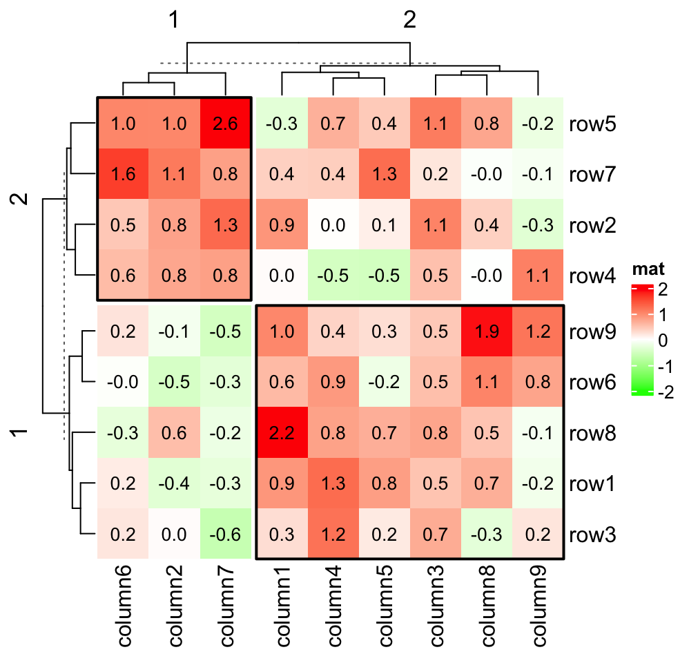
You can split the heatmap without doing anything extra to cell_fun:
Heatmap(small_mat, name = "mat", col = col_fun,
    row_km = 2, column_km = 2,
    cell_fun = function(j, i, x, y, width, height, fill) {
        grid.text(sprintf("%.1f", small_mat[i, j]), x, y, gp = gpar(fontsize = 10))
})
In following example, we make a heatmap which shows correlation matrix similar as the corrplot package:
cor_mat = cor(small_mat)
od = hclust(dist(cor_mat))$order
cor_mat = cor_mat[od, od]
nm = rownames(cor_mat)
col_fun = circlize::colorRamp2(c(-1, 0, 1), c("green", "white", "red"))
# `col = col_fun` here is used to generate the legend
Heatmap(cor_mat, name = "correlation", col = col_fun, rect_gp = gpar(type = "none"),
    cell_fun = function(j, i, x, y, width, height, fill) {
        grid.rect(x = x, y = y, width = width, height = height,
            gp = gpar(col = "grey", fill = NA))
        if(i == j) {
            grid.text(nm[i], x = x, y = y)
        } else if(i > j) {
            grid.circle(x = x, y = y, r = abs(cor_mat[i, j])/2 * min(unit.c(width, height)),
                gp = gpar(fill = col_fun(cor_mat[i, j]), col = NA))
        } else {
            grid.text(sprintf("%.1f", cor_mat[i, j]), x, y, gp = gpar(fontsize = 10))
        }
    }, cluster_rows = FALSE, cluster_columns = FALSE,
    show_row_names = FALSE, show_column_names = FALSE)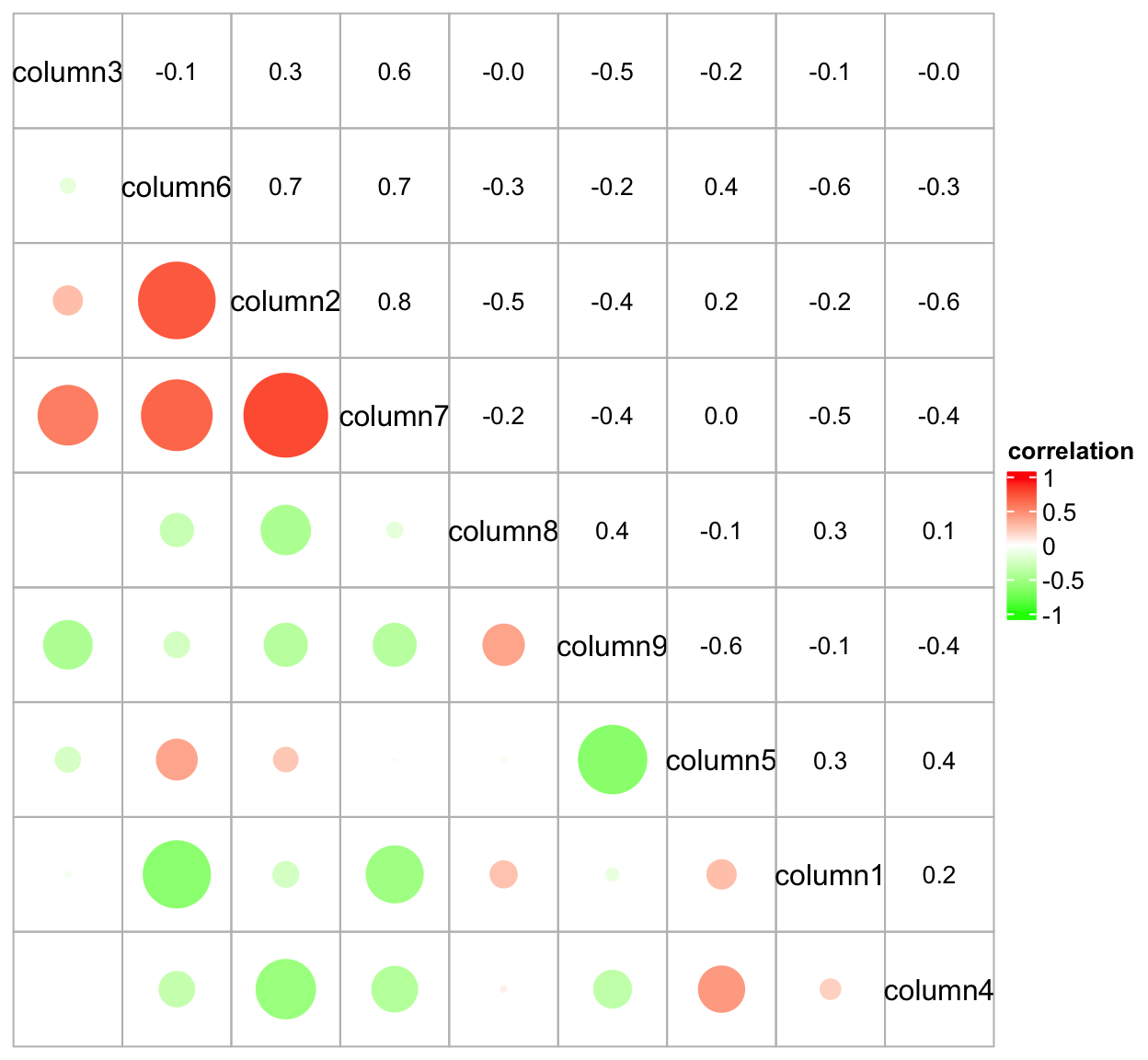
As you may see in previous plot, when setting the non-standard parameter
rect_gp = gpar(type = "none"), the clustering is performed but nothing is
drawn on the heatmap body.
One last example is to visualize a GO game. The input data takes records of moves in the game.
str = [1615 chars quoted with '"']We convert it into a matrix:
str = gsub("\\n", "", str)
step = strsplit(str, ";")[[1]]
type = gsub("(B|W).*", "\\1", step)
row = gsub("(B|W)\\[(.).\\]", "\\2", step)
column = gsub("(B|W)\\[.(.)\\]", "\\2", step)

go_mat = matrix(nrow = 19, ncol = 19)
rownames(go_mat) = letters[1:19]
colnames(go_mat) = letters[1:19]
for(i in seq_along(row)) {
    go_mat[row[i], column[i]] = type[i]
}
go_mat[1:4, 1:4]
## a b c d
## a NA NA NA "W"
## b "W" "W" "W" "B"
## c "B" "B" "W" "W"
## d "B" "W" "B" "W"Black and white stones are put based on the values in the matrix:
ht = Heatmap(go_mat, name = "go", rect_gp = gpar(type = "none"),
    cell_fun = function(j, i, x, y, w, h, col) {
        grid.rect(x, y, w, h, gp = gpar(fill = "#dcb35c", col = NA))
        if(i == 1) {
            grid.segments(x, y-h*0.5, x, y)
        } else if(i == nrow(go_mat)) {
            grid.segments(x, y, x, y+h*0.5)
        } else {
            grid.segments(x, y-h*0.5, x, y+h*0.5)
        }
        if(j == 1) {
            grid.segments(x, y, x+w*0.5, y)
        } else if(j == ncol(go_mat)) {
            grid.segments(x-w*0.5, y, x, y)
        } else {
            grid.segments(x-w*0.5, y, x+w*0.5, y)
        }

        if(i %in% c(4, 10, 16) & j %in% c(4, 10, 16)) {
            grid.points(x, y, pch = 16, size = unit(2, "mm"))
        }

        r = min(unit.c(w, h))*0.45
        if(is.na(go_mat[i, j])) {
        } else if(go_mat[i, j] == "W") {
            grid.circle(x, y, r, gp = gpar(fill = "white", col = "white"))
        } else if(go_mat[i, j] == "B") {
            grid.circle(x, y, r, gp = gpar(fill = "black", col = "black"))
        }
    },
    col = c("B" = "black", "W" = "white"),
    show_row_names = FALSE, show_column_names = FALSE,
    column_title = "One famous GO game",
    show_heatmap_legend = FALSE
)
lgd = Legend(title = "Players", labels = c("player1", "player2"),
    type = "points", legend_gp = gpar(col = c("black", "white")),
    size = unit(0.45, "snpc"), background = "#dcb35c")
draw(ht, heatmap_legend_list = lgd)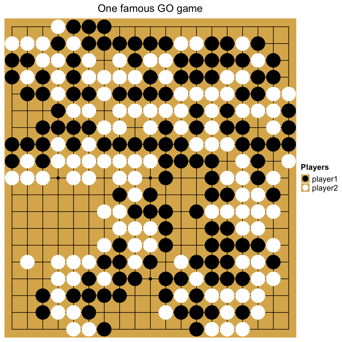
In the Go game example, we actually self-defined a legend. This will be introduced in Section 5 in more details.
2.9.2 layer_fun
If you tried out the previous code for the Go game, you might see the generation of
the plot is a little bit slow that fragments in the plot come one after other other.
This is because cell_fun is applied in every cell separately. In this section,
we will introduce layer_fun which is a vectorized version of cell_fun.
cell_fun adds graphics cell by cell, while layer_fun adds graphics in a
block-wise manner. Similar as cell_fun, layer_fun also needs seven
arguments, but they are all in vector form (layer_fun can also have a eighth and
ninth arguments which is introduced later in this section):
# code only for demonstration
Heatmap(..., layer_fun = function(j, i, x, y, w, h, fill) {...})
# or you can capitalize the arguments to mark they are vectors,
# the names of the argument do not matter
Heatmap(..., layer_fun = function(J, I, X, Y, W, H, F) {...})
j and i still contain the column and row indices corresponding to the
original matrix, but since now layer_fun is applied to a heatmap slice which
contains a block of cells, j and i are vectors for all the cells in the
current heatmap slice. Similarlly, x, y, w, h and fill are all vectors
corresponding to all cells in the current heatmap slice.
Since j and i now are vectors, to get corresponding values in the matrix, we
cannot use the form as mat[j, i] because it gives you a sub-matrix with
length(i) rows and length(j) columns. Instead we can use pindex()
function from ComplexHeatmap which is like pairwise indexing for a matrix.
See follow example:
##      [,1] [,2]
## [1,]    1    7
## [2,]    2    8
# but we actually want mfoo[1, 1] and mfoo[2, 3]
pindex(mfoo, 1:2, c(1, 3))
## [1] 1 8Next example shows the layer_fun version of adding text on heatmap. It’s
basically the same as the cell_fun version.
col_fun = colorRamp2(c(-2, 0, 2), c("green", "white", "red"))
Heatmap(small_mat, name = "mat", col = col_fun,
    layer_fun = function(j, i, x, y, width, height, fill) {
        # since grid.text can also be vectorized
        grid.text(sprintf("%.1f", pindex(small_mat, i, j)), x, y,
            gp = gpar(fontsize = 10))
})
And only add text to cells with positive values:
Heatmap(small_mat, name = "mat", col = col_fun,
    layer_fun = function(j, i, x, y, width, height, fill) {
        v = pindex(small_mat, i, j)
        l = v > 0
        grid.text(sprintf("%.1f", v[l]), x[l], y[l], gp = gpar(fontsize = 10))
})
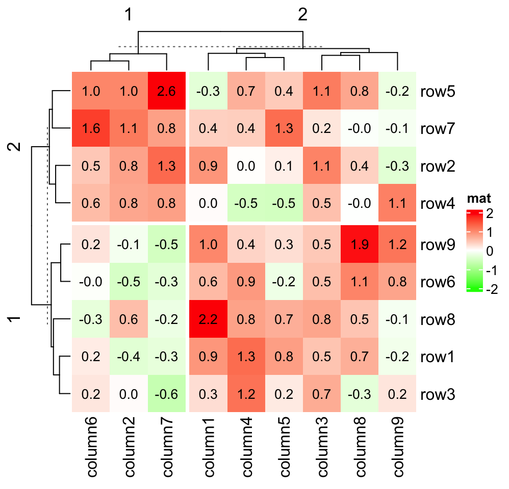
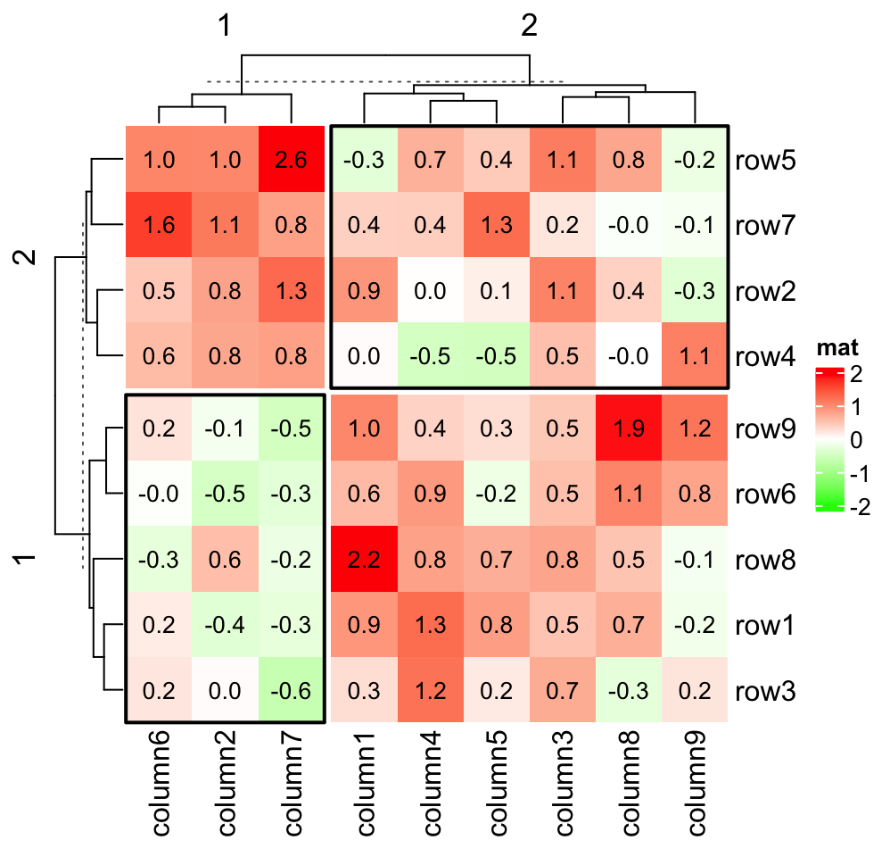
When the heatmap is split, layer_fun is applied in every slice.
Heatmap(small_mat, name = "mat", col = col_fun,
    row_km = 2, column_km = 2,
    layer_fun = function(j, i, x, y, width, height, fill) {
        v = pindex(small_mat, i, j)
        grid.text(sprintf("%.1f", v), x, y, gp = gpar(fontsize = 10))
        if(sum(v > 0)/length(v) > 0.75) {
            grid.rect(gp = gpar(lwd = 2, fill = "transparent"))
        }
})
layer_fun can also have two more arguments which are the index for the
current row slice and column slice. E.g. we want to add borders for the top
right and bottom left slices.
Heatmap(small_mat, name = "mat", col = col_fun,
    row_km = 2, column_km = 2,
    layer_fun = function(j, i, x, y, width, height, fill, slice_r, slice_c) {
        v = pindex(small_mat, i, j)
        grid.text(sprintf("%.1f", v), x, y, gp = gpar(fontsize = 10))
        if(slice_r != slice_c) {
            grid.rect(gp = gpar(lwd = 2, fill = "transparent"))
        }
})
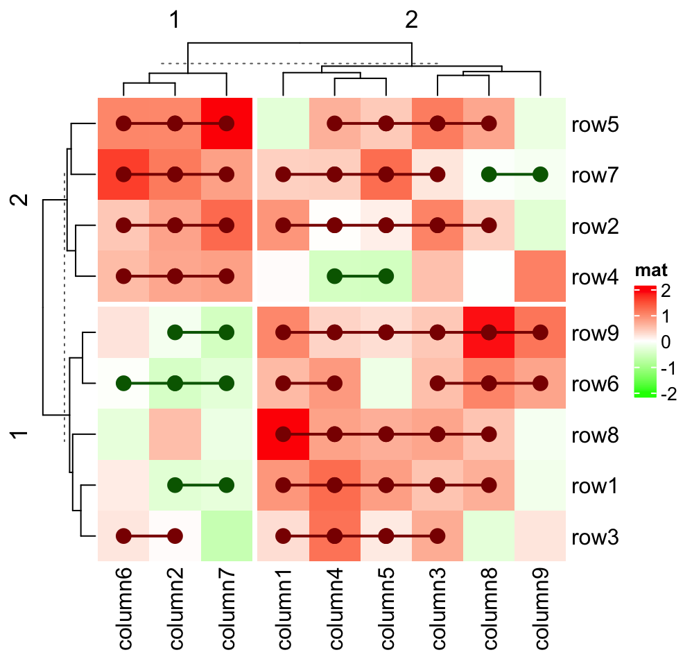
The advantage of layer_fun is that it is not only fast to add graphics, but
also it provides more possibilities to customize the heatmap, e.g. you can
interact between cells in a heatmap slice. Consider following visualization: For
each row in the heatmap, if values in the neighbouring two columns have the same
sign, we add a red line or a green line depending on the sign of the two values.
Since now graphics in a cell depend on other cells, it is only possible to
implement it via layer_fun. (Don’t be frightened by following code. They are
explained after the code.)
Heatmap(small_mat, name = "mat", col = col_fun,
    row_km = 2, column_km = 2,
    layer_fun = function(j, i, x, y, w, h, fill) {
        # restore_matrix() is explained after this chunk of code
        ind_mat = restore_matrix(j, i, x, y)
        for(ir in seq_len(nrow(ind_mat))) {
            # start from the second column
            for(ic in seq_len(ncol(ind_mat))[-1]) {
                ind1 = ind_mat[ir, ic-1] # previous column
                ind2 = ind_mat[ir, ic]   # current column
                v1 = small_mat[i[ind1], j[ind1]]
                v2 = small_mat[i[ind2], j[ind2]]
                if(v1 * v2 > 0) { # if they have the same sign
                    col = ifelse(v1 > 0, "darkred", "darkgreen")
                    grid.segments(x[ind1], y[ind1], x[ind2], y[ind2],
                        gp = gpar(col = col, lwd = 2))
                    grid.points(x[c(ind1, ind2)], y[c(ind1, ind2)],
                        pch = 16, gp = gpar(col = col), size = unit(4, "mm"))
                }
            }
        }
    }
)
The values that are sent to layer_fun are all vectors (for the vectorization
of the grid graphics functions), however, the heatmap slice where
layer_fun is applied to, is still represented by a matrix, thus, it would be
very convinient if all the arguments in layer_fun can be converted to the
sub-matrix for the current slice. Here, as shown in above example,
restore_matrix() does the job. restore_matrix() directly accepts the first
four argument in layer_fun and returns an index matrix, where rows and
columns correspond to the rows and columns in the current slice, from top to
bottom and from left to right. The values in the matrix are the natural order
of e.g. vector j in current slice.
If you run following code:
Heatmap(small_mat, name = "mat", col = col_fun,
    row_km = 2, column_km = 2,
    layer_fun = function(j, i, x, y, w, h, fill) {
        ind_mat = restore_matrix(j, i, x, y)
        print(ind_mat)
    }
)
The first output which is for the top-left slice:
     [,1] [,2] [,3] [,4] [,5]
[1,]    1    4    7   10   13
[2,]    2    5    8   11   14
[3,]    3    6    9   12   15
As you see, this is a three-row and five-column index matrix where the first
row corresponds to the top row in the slice. The values in the matrix
correspond to the natural index (i.e. 1, 2, …) in j, i, x, y,
… in layer_fun. Now, if we want to add values on the second column in the
top-left slice, the code which is put inside layer_fun would look like:
for(ind in ind_mat[, 2]) {
grid.text(small_mat[i[ind], j[ind]], x[ind], y[ind], ...)
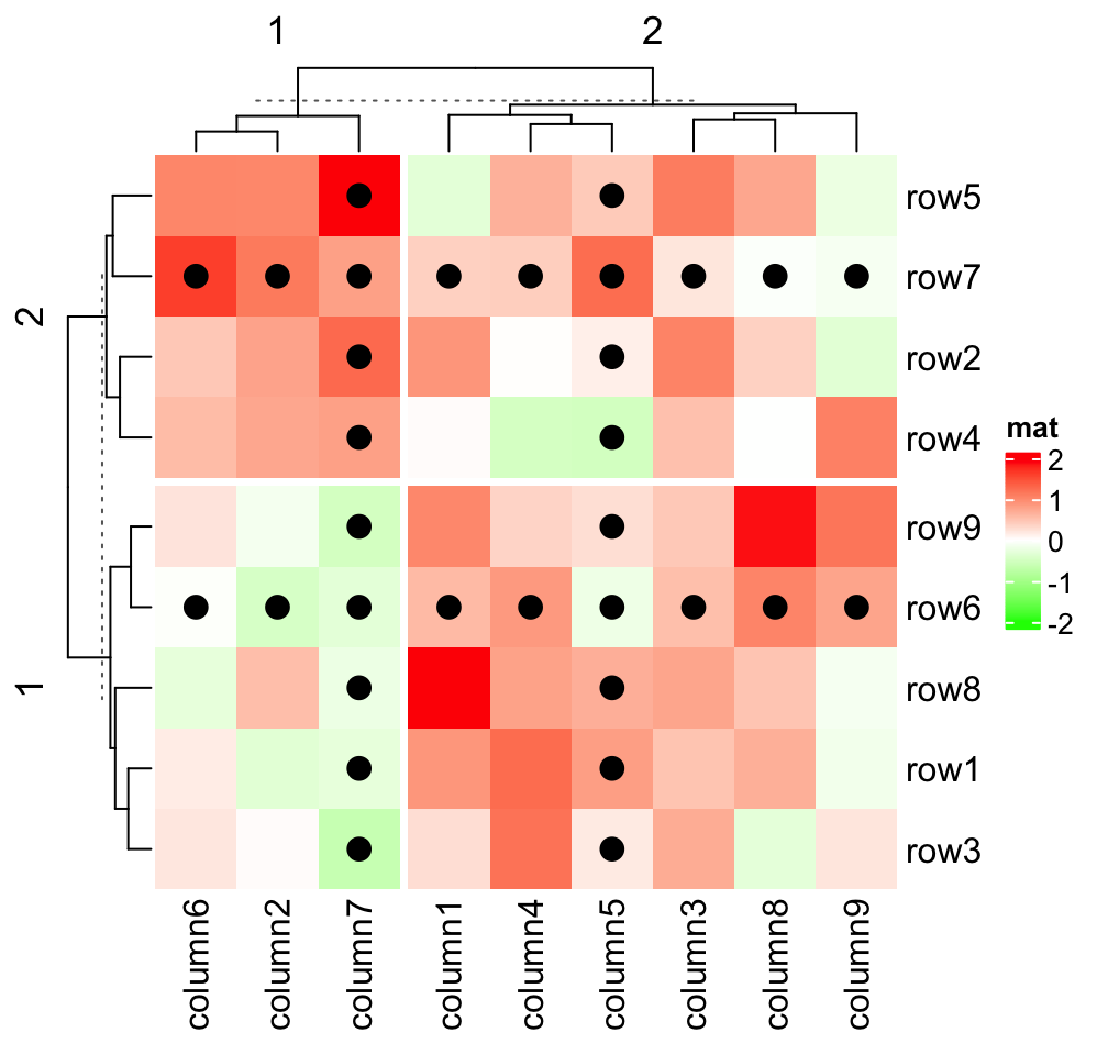
}Now it is easier to understand the second example: we want to add points to the second row and the third column in every slice:
Heatmap(small_mat, name = "mat", col = col_fun,
    row_km = 2, column_km = 2,
    layer_fun = function(j, i, x, y, w, h, fill) {
        ind_mat = restore_matrix(j, i, x, y)
        ind = unique(c(ind_mat[2, ], ind_mat[, 3]))
        grid.points(x[ind], y[ind], pch = 16, size = unit(4, "mm"))
    }
)
2.10 Size of the heatmap
width, heatmap_width, height and heatmap_height control the size of
the heatmap. By default, all heatmap components have fixed width or height,
e.g. the width of row dendrogram is 1cm. The width or the height of the
heatmap body fill the rest area of the final plotting region, which means, if
you draw it in an interactive graphic window and you change the size of the
window by draging it, the size of the heatmap body is automatically adjusted.
heatmap_width and heatmap_height control the width/height of the complete
heatmap including all heatmap components (excluding the legends) while width
and height only control the width/height of the heamtap body. All these four
arguments can be set as absolute units.
Heatmap(mat, name = "mat", width = unit(8, "cm"), height = unit(8, "cm"))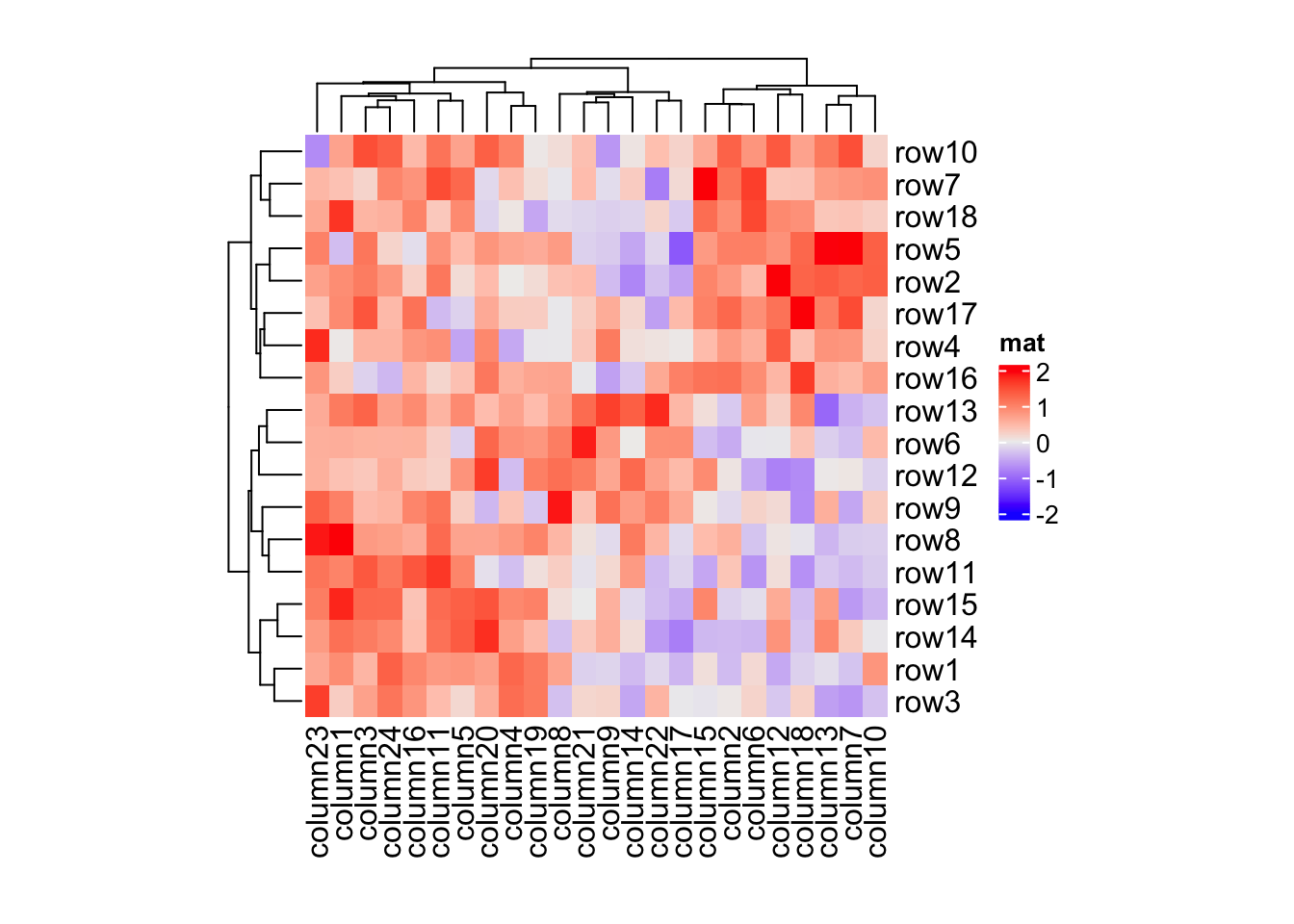
Heatmap(mat, name = "mat", heatmap_width = unit(8, "cm"),
    heatmap_height = unit(8, "cm"))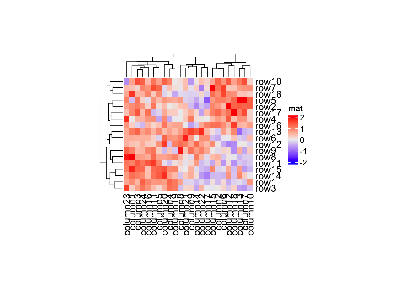
These four arguments are more important when adjust the size in a list of heatmaps (see Section 4.2).
When the size of the heatmap is set as absolute units, it is possible that the
size of the figure is larger than the size of the heatmap, which gives blank
areas around the heatmap. The size of the heatmap can be retrieved by ComplexHeatmap:::width()
and ComplexHeatmap:::height() functions.
ht = Heatmap(mat, name = "mat", width = unit(8, "cm"), height = unit(8, "cm"))
ht = draw(ht) # you must call draw() to reassign the heatmap variable
ComplexHeatmap:::width(ht)
## [1] 118.851591171994mm
ComplexHeatmap:::height(ht)## [1] 114.717557838661mm
ht = Heatmap(mat, name = "mat", heatmap_width = unit(8, "cm"),
    heatmap_height = unit(8, "cm"))
ht = draw(ht)
ComplexHeatmap:::width(ht)
## [1] 94.8877245053272mm
ComplexHeatmap:::height(ht)## [1] 83.8660578386606mmCheck this blog post (Set cell width/height in the heatmap) if you want to save the heatmap in a figure file which has exactly the same size as the heatmap.
2.11 Plot the heatmap
Heatmap() function actually is only a constructor, which means it only puts
all the data and configurations into the object in the Heatmap class. The
clustering will only be performed when the draw() method is called. Under
interactive mode (e.g. the interactive R terminal where you can type your R
code line by line), directly calling Heatmap() without assigning to any
object prints the object and the print method (or the S4 show() method) for
the Heatmap class object calls draw() internally. So if you type
Heatmap(...) in your R terminal, it looks like it is a plotting function
like plot(), you need to be aware of that it is actually not true and in the
following cases you might see nothing plotted.
- you put
Heatmap(...)inside a function, - you put
Heatmap(...)in a code chunk likefororif-else - you put
Heatmap(...)in an Rscript and you run it under command line.
The reason is in above three cases, the show() method WILL NOT be called and
thus draw() method is not executed either. So, to make the plot, you need to
call draw() explicitly: draw(Heatmap(...)) or:
# code only for demonstration
ht = Heatmap(...)
draw(ht)
The draw() function actually is applied to a list of heatmaps in
HeatmapList class. The draw() method for the single Heatmap class
constructs a HeatmapList with only one heatmap and call draw() method of
the HeatmapList class. The draw() function accpets a lot of more arguments
which e.g. control the legends. It will be discussed in Chapter
4.
draw(ht, heatmap_legend_side, padding, ...)2.12 Extract orders and dendrograms
The row/column orders of the heatmap can be obtained by
row_order()/column_order() functions. You can directly apply to the
heatmap object returned by Heatmap() or to the object returned by draw().
In following, we take row_order() as example.
small_mat = mat[1:9, 1:9]
ht1 = Heatmap(small_mat)
row_order(ht1)
## [1] 5 7 2 4 9 6 8 1 3
ht2 = draw(ht1)
row_order(ht2)
## [1] 5 7 2 4 9 6 8 1 3As explained in previous section, Heatmap() function does not perform
clustering, thus, when directly apply row_order() on ht1, clustering will
be first performed. Later when making the heatmap by draw(ht1), the
clustering will be applied again. This might be a problem that if you set
k-means clustering in the heatmap. Since the clustering is applied twice,
k-means might give you different clusterings, which means, you might have
different results from row_order() and you might have different heatmap.
In following chunk of code, o1, o2 and o3 might be different because
each time, k-means clustering is performed.
# code only for demonstration
ht1 = Heatmap(small_mat, row_km = 2)
o1 = row_order(ht1)
o2 = row_order(ht1)
ht2 = draw(ht1)
o3 = row_order(ht2)
o4 = row_order(ht2)
draw() function returns the heatmap (or more precisely, the heatmap list)
which has already been reordered, and applying row_order() just extracts the
row order from the object, which ensures the row order is exactly the same as
the one shown in the heatmap. In above code, o3 is always identical to o4.
So, the preferable way to get row/column orders is as follows.
# code only for demonstration
ht = Heatmap(small_mat)
ht = draw(ht)
row_order(ht)
column_order(ht)
If rows/columns are split, row order or column order will be a list.
ht = Heatmap(small_mat, row_km = 2, column_km = 3)
ht = draw(ht)
row_order(ht)
## $`2`
## [1] 5 7 2 4
##
## $`1`
## [1] 9 6 8 1 3
column_order(ht)## $`1`
## [1] 6 2 7
##
## $`3`
## [1] 1 3 4 5
##
## $`2`
## [1] 8 9Similarly, the row_dend()/column_dend() functions return the dendrograms.
It returns a single dendrogram or a list of dendrograms depending on whether
the heatmap is split.
ht = Heatmap(small_mat, row_km = 2)
ht = draw(ht)
row_dend(ht)
## $`2`
## 'dendrogram' with 2 branches and 4 members total, at height 2.946428
##
## $`1`
## 'dendrogram' with 2 branches and 5 members total, at height 2.681351
column_dend(ht)## 'dendrogram' with 2 branches and 9 members total, at height 4.574114row_order(), column_order(), row_dend() and column_dend() also work
for a list of heatmaps, it will be introduced in Section
4.12.
2.13 Subset a heatmap
Since heatmap is a representation of a matrix, there is also a subset method
for the Heatmap class.
ht = Heatmap(mat, name = "mat")
dim(ht)
## [1] 18 24
ht[1:10, 1:10]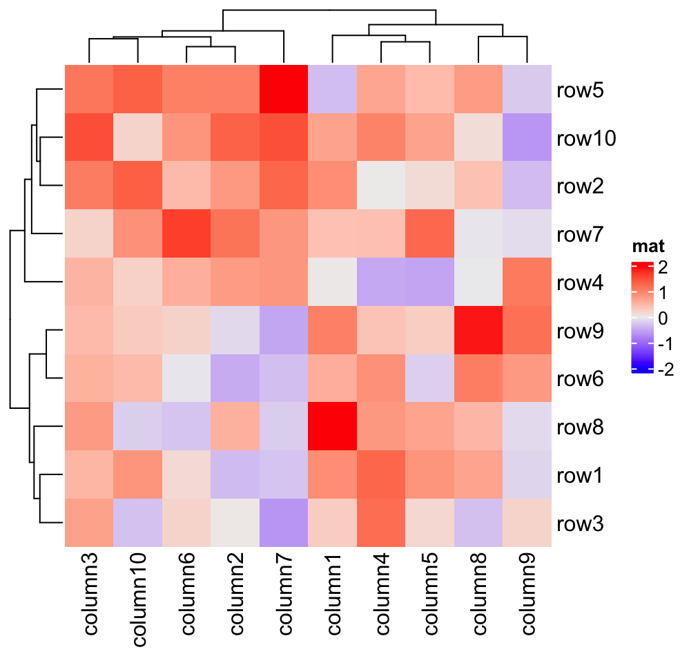
The annotations are subsetted accordingly as well.
ht = Heatmap(mat, name = "mat", row_km = 2, column_km = 3,
    col = colorRamp2(c(-2, 0, 2), c("green", "white", "red")),
    top_annotation = HeatmapAnnotation(foo1 = 1:24, bar1 = anno_points(runif(24))),
    right_annotation = rowAnnotation(foo2 = 18:1, bar2 = anno_barplot(runif(18)))
)
ht[1:9*2 - 1, 1:12*2] # odd rows, even columns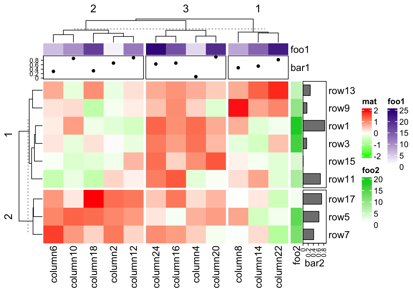
The heatmap components are subsetted if they are vector-like. Some
configurations in the heatmap keep the same when subsetting, e.g. if row_km
is set in the original heatmap, the configuration of k-means is kept and it is
performed in the sub-heatmap. So in following example, k-means clustering is
only performed when making heatmap for ht2.
ht = Heatmap(mat, name = "mat", row_km = 2)
ht2 = ht[1:10, 1:10]
ht2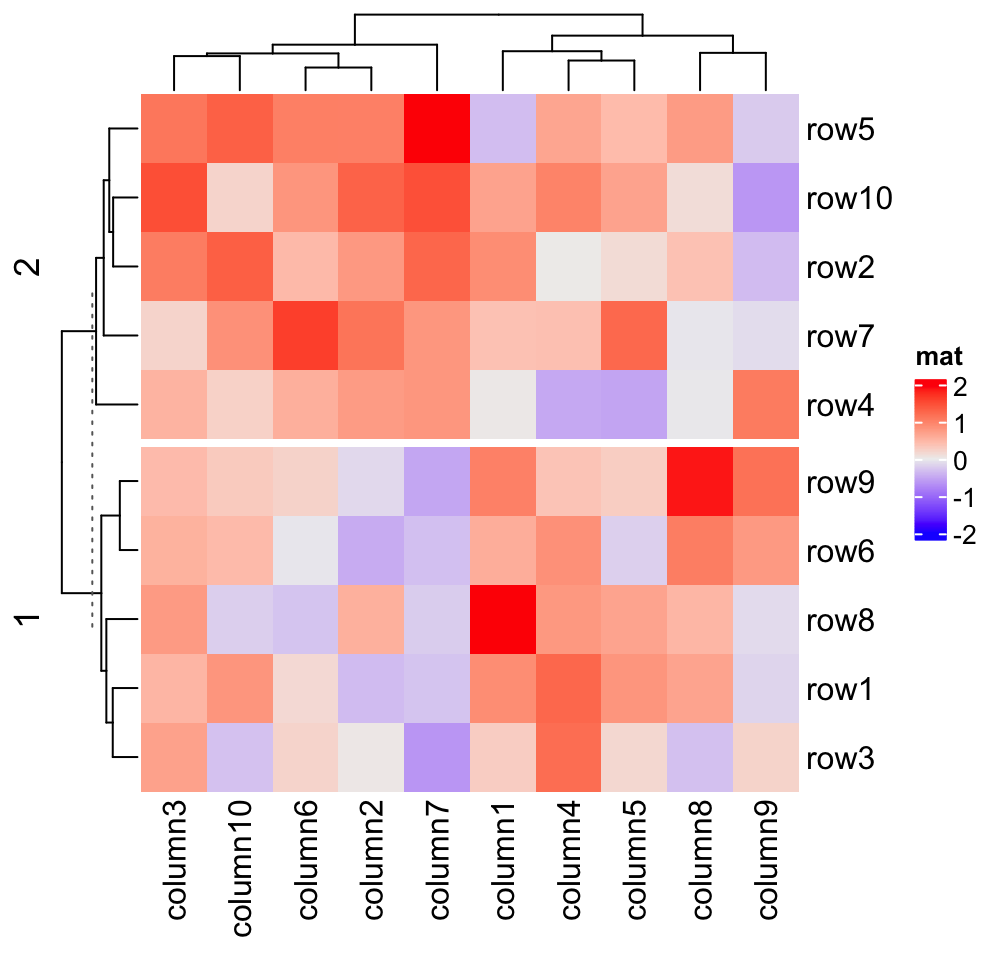
The implementation of subsetting heatmaps is very experimental. It is not
always working, e.g. if cell_fun is defined and uses an external matrix, or
clustering objects are assigned to cluster_rows or cluster_columns.
There are also subset methods for the HeatmapAnnotation class (Section
3.22) and the HeatmapList class (Section 4.10),
but both are very experimental as well.