Chapter 11 modes for `circos.genomicTrack()`

The behaviour of circos.genomicTrack() and panel.fun will be different according to different input data (e.g. is it a simple data frame or a list of data frames? If it is a data frame, how many numeric columns it has?) and different settings.

11.1 Normal mode

11.1.1 Input is a data frame

If input data is a data frame in BED format, region in panel.fun would be a data frame containing start position and end position in the current chromosome which is extracted from data. value is also a data frame which contains columns in data excluding the first three columns. Index of proper numeric columns will be passed by ... if it is set in circos.genomicTrack(). If users want to use such information, they need to pass ... to low-level genomic function such as circos.genoimcPoints() as well.

If there are more than one numeric columns, graphics are added for each column repeatedly (with same genomic positions).

data = generateRandomBed(nc = 2)
circos.genomicTrack(data, numeric.column = 4, 
    panel.fun = function(region, value, ...) {
        circos.genomicPoints(region, value, ...)
        circos.genomicPoints(region, value)
        # 1st column in `value` while 4th column in `data`
        circos.genomicPoints(region, value, numeric.column = 1)
})

11.1.2 Input is a list of data frames

If input data is a list of data frames, panel.fun is applied on each data frame iteratively to the current cell. Under such condition, region and value will contain corresponding data in the current data frame and in the current chromosome. The index for the current data frame can be get by getI(...). Note getI(...) can only be used inside panel.fun and ... argument is mandatory.

When numeric.column is specified in circos.genomicTrack(), the length of numeric.column can only be one or the number of data frames, which means, there is only one numeric column that will be used in each data frame. If it is not specified, the first numeric column in each data frame is used.

bed_list = list(generateRandomBed(), generateRandomBed())
circos.genomicTrack(bed_list,
    panel.fun = function(region, value, ...) {
        i = getI(...)
        circos.genomicPoints(region, value, col = i, ...)
})

# column 4 in the first bed and column 5 in the second bed
circos.genomicTrack(bed_list, numeric.column = c(4, 5),
    panel.fun = function(region, value, ...) {
        i = getI(...)
        circos.genomicPoints(region, value, col = i, ...)
})

11.2 Stack mode

circos.genomicTrack() also supports a stack mode by setting stack = TRUE. Under stack mode, ylim is re-defined inside the function and the y-axis is splitted into several bins with equal height and graphics are put onto “horizontal” bins (with position y = 1, 2, ...).

11.2.1 Input is a data frame

Under stack mode, when input data is a single data frame containing one or more numeric columns, each numeric column defined in numeric.column will be treated as a single unit (recall that when numeric.column is not specified, all numeric columns are used). ylim is re-defined to c(0.5, n+0.5) in which n is number of numeric columns specified. panel.fun is applied iteratively on each numeric column and add graphics to the horizontal line y = i. In this case, actually value in e.g. circos.genomicPoints() doesn’t used for mapping the y positions, while replaced with y = i internally.

In each iteration, in panel.fun, region is still the genomic regions in current chromosome, but value only contains current numeric column plus all non-numeric columns. The value of the index of “current” numeric column can be obtained by getI(...).

data = generateRandomBed(nc = 2)
circos.genomicTrack(data, stack = TRUE,
    panel.fun = function(region, value, ...) {
        i = getI(...)
        circos.genomicPoints(region, value, col = i, ...)
})

11.2.2 Input is a list of data frames

When input data is a list of data frames, each data frame will be treated as a single unit. ylim is re-defined to c(0.5, n+0.5) in which n is the number of data frames. panel.fun will be applied iteratively on each data frame. In each iteration, in panel.fun, region is still the genomic regions in current chromosome, and value contains columns in current data frame excluding the first three columns. Graphics by low-level genomic functions will be added on the `horizontal’ bins.

bed_list = list(generateRandomBed(), generateRandomBed())
circos.genomicTrack(bed_list, stack = TRUE,
    panel.fun = function(region, value, ...) {
        i = getI(...)
        circos.genomicPoints(region, value, ...)
})

Under stack mode, if using a data frame with multiple numeric columns, graphics on all horizontal bins share the same genomic positions while if using a list of data frames, the genomic positions can be different.

11.3 Applications

In this section, we will show several real examples of adding genomic graphics under different modes. Again, if you are not happy with these functionalities, you can simply re-implement your plot with the basic circlize functions.

11.3.1 Points

To make plots more clear to look at, we only add graphics in the first quarter of the circle and initialize the plot only with chromosome 1.

set.seed(999)
circos.par("track.height" = 0.1, start.degree = 90,
    canvas.xlim = c(0, 1), canvas.ylim = c(0, 1), gap.degree = 270)
circos.initializeWithIdeogram(chromosome.index = "chr1", plotType = NULL)

In the example figure (Figure 11.1) below, each track contains points under different modes.

In track A, it is the most normal way to add points. Here bed only contains one numeric column and points are added at the middle points of regions.

bed = generateRandomBed(nr = 300)
circos.genomicTrack(bed, panel.fun = function(region, value, ...) {
    circos.genomicPoints(region, value, pch = 16, cex = 0.5, ...)
})

In track B, if it is specified as stack mode, points are added in a horizontal line (or visually, a circular line).

circos.genomicTrack(bed, stack = TRUE, 
    panel.fun = function(region, value, ...) {
        circos.genomicPoints(region, value, pch = 16, cex = 0.5,...)
        i = getI(...)
        circos.lines(CELL_META$cell.xlim, c(i, i), lty = 2, col = "#00000040")
})

In track C, the input data is a list of two data frames. panel.fun is applied iterately on each data frame. The index of “current” index can be obtained by getI(...).

bed1 = generateRandomBed(nr = 300)
bed2 = generateRandomBed(nr = 300)
bed_list = list(bed1, bed2)
circos.genomicTrack(bed_list, 
    panel.fun = function(region, value, ...) {
        i = getI(...)
        circos.genomicPoints(region, value, pch = 16, cex = 0.5, col = i, ...)
})

In track D, the list of data frames is plotted under stack mode. Graphics corresponding to each data frame are added to a horizontal line.

circos.genomicTrack(bed_list, stack = TRUE, 
    panel.fun = function(region, value, ...) {
        i = getI(...)
        circos.genomicPoints(region, value, pch = 16, cex = 0.5, col = i, ...)
        circos.lines(CELL_META$cell.xlim, c(i, i), lty = 2, col = "#00000040")
})

In track E, the data frame has four numeric columns. Under normal mode, all the four columns are used with the same genomic coordinates.

bed = generateRandomBed(nr = 300, nc = 4)
circos.genomicTrack(bed, 
    panel.fun = function(region, value, ...) {
        circos.genomicPoints(region, value, pch = 16, cex = 0.5, col = 1:4, ...)
})

In track F, the data frame has four columns but is plotted under stack mode. Graphics for each column are added to a horizontal line. Current column can be obtained by getI(...). Note here value in panel.fun is a data frame with only one column (which is the current numeric column).

bed = generateRandomBed(nr = 300, nc = 4)
circos.genomicTrack(bed, stack = TRUE, 
    panel.fun = function(region, value, ...) {
        i = getI(...)
        circos.genomicPoints(region, value, pch = 16, cex = 0.5, col = i, ...)
        circos.lines(CELL_META$cell.xlim, c(i, i), lty = 2, col = "#00000040")
})
circos.clear()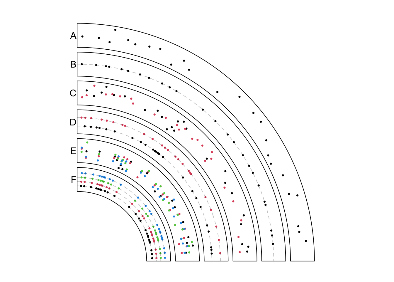

Figure 11.1: Add points under different modes.

11.3.2 Lines

Similar as previous figure, only the first quarter in the circle is visualized. Examples are shown in Figure 11.2.

circos.par("track.height" = 0.08, start.degree = 90,
    canvas.xlim = c(0, 1), canvas.ylim = c(0, 1), gap.degree = 270,
    cell.padding = c(0, 0, 0, 0))
circos.initializeWithIdeogram(chromosome.index = "chr1", plotType = NULL)

In track A, it is the most simple way to add lines. Middle points of regions are used as the values on x-axes.

bed = generateRandomBed(nr = 500)
circos.genomicTrack(bed, 
    panel.fun = function(region, value, ...) {
        circos.genomicLines(region, value)
})

circos.genomicLines() is implemented by circos.lines(), thus, arguments supported in circos.lines() can also be in circos.genomicLines(). In track B, the area under the line is filled with color and in track C, type of the line is set to h.

circos.genomicTrack(bed, 
    panel.fun = function(region, value, ...) {
        circos.genomicLines(region, value, area = TRUE)
})
circos.genomicTrack(bed, 
    panel.fun = function(region, value, ...) {
        circos.genomicLines(region, value, type = "h")
})

In track D, the input is a list of data frames. panel.fun is applied to each data frame iterately.

bed1 = generateRandomBed(nr = 500)
bed2 = generateRandomBed(nr = 500)
bed_list = list(bed1, bed2)
circos.genomicTrack(bed_list, 
    panel.fun = function(region, value, ...) {
        i = getI(...)
        circos.genomicLines(region, value, col = i, ...)
})

In track E, the input is a list of data frames and is drawn under stack mode. Each genomic region is drawn as a horizontal segment and is put on a horizontal line where the width of the segment corresponds to the width of the genomc region. Under stack mode, for circos.genomicLines(), type of lines is only restricted to segments.

circos.genomicTrack(bed_list, stack = TRUE, 
    panel.fun = function(region, value, ...) {
        i = getI(...)
        circos.genomicLines(region, value, col = i, ...)
})

In track F, the input is a data frame with four numeric columns. Each column is drawn under the normal mode where the same genomic coordinates are shared.

bed = generateRandomBed(nr = 500, nc = 4)
circos.genomicTrack(bed, 
    panel.fun = function(region, value, ...) {
        circos.genomicLines(region, value, col = 1:4, ...)
})

In track G, the data frame with four numeric columns are drawn under stack mode. All the four columns are drawn to four horizontal lines.

bed = generateRandomBed(nr = 500, nc = 4)
circos.genomicTrack(bed, stack = TRUE, 
    panel.fun = function(region, value, ...) {
        i = getI(...)
        circos.genomicLines(region, value, col = i, ...)
})

In track H, we specify type to segment and set different colors for segments. Note each segment is located at the y position defined in the numeric column.

bed = generateRandomBed(nr = 200)
circos.genomicTrack(bed, 
    panel.fun = function(region, value, ...) {
        circos.genomicLines(region, value, type = "segment", lwd = 2, 
            col = rand_color(nrow(region)), ...)
})
circos.clear()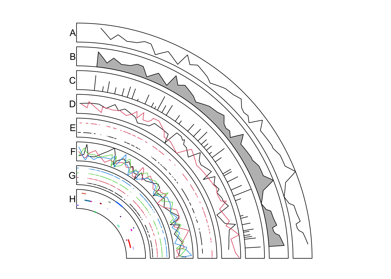

Figure 11.2: Add lines under different modes.

11.3.3 Rectangles

Again, only the first quarter of the circle is initialized. For rectangles, the filled colors are always used to represent numeric values. Here we define a color mapping function col_fun to map values to colors. Examples are in Figure 11.3.

circos.par("track.height" = 0.15, start.degree = 90,
    canvas.xlim = c(0, 1), canvas.ylim = c(0, 1), gap.degree = 270)
circos.initializeWithIdeogram(chromosome.index = "chr1", plotType = NULL)
col_fun = colorRamp2(breaks = c(-1, 0, 1), colors = c("green", "black", "red"))

To draw heatmaps, you probably want to use the stack mode. In track A, bed has four numeric columns and stack mode is used to arrange the heatmap. You can see rectangles are stacked for a certain genomic region.

bed = generateRandomBed(nr = 100, nc = 4)
circos.genomicTrack(bed, stack = TRUE, 
    panel.fun = function(region, value, ...) {
        circos.genomicRect(region, value, col = col_fun(value[[1]]), border = NA, ...)
})

In track B, the input is a list of data frames. Under stack mode, each data frame is added to a horizontal line. Since genomic positions for different data frames can be different, you may see in the figure, positions for the two sets of rectangles are different.

Under stack mode, by default, the height of rectangles is internally set to make them completely fill the cell in the vertical direction. ytop and ybottom can be used to adjust the height of rectangles. Note each line of rectangles is at y = i and the default height of rectangles are 1.

bed1 = generateRandomBed(nr = 100)
bed2 = generateRandomBed(nr = 100)
bed_list = list(bed1, bed2)
circos.genomicTrack(bed_list, stack = TRUE, 
    panel.fun = function(region, value, ...) {
        i = getI(...)
        circos.genomicRect(region, value, ytop = i + 0.3, ybottom = i - 0.3,
            col = col_fun(value[[1]]), ...)
})

In track C, we implement same graphics as in track B, but with the normal mode. Under stack mode, data range on y axes and positions of rectangles are adjusted internally. Here we explicitly adjust it under the normal mode.

circos.genomicTrack(bed_list, ylim = c(0.5, 2.5), 
    panel.fun = function(region, value, ...) {
        i = getI(...)
        circos.genomicRect(region, value, ytop = i + 0.3, ybottom = i - 0.3, 
            col = col_fun(value[[1]]), ...)
})

In track D, rectangles are used to make barplots. We specify the position of the top of bars by ytop.column (1 means the first column in value).

bed = generateRandomBed(nr = 200)
circos.genomicTrack(bed, 
    panel.fun = function(region, value, ...) {
        circos.genomicRect(region, value, ytop.column = 1, ybottom = 0, 
            col = ifelse(value[[1]] > 0, "red", "green"), ...)
        circos.lines(CELL_META$cell.xlim, c(0, 0), lty = 2, col = "#00000040")
})
circos.clear()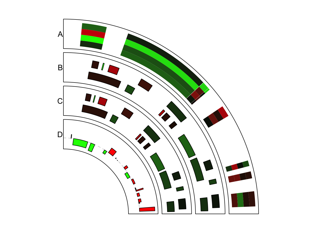

Figure 11.3: Add rectangles under different modes.

Chapter 11 modes for circos.genomicTrack()