Topic 1-01: GO gene sets

To obtain GO gene sets, we need to use two packages: GO.db and org.*.db packages.

The GO.db package

We first load the package.

library(GO.db)

GO data is represented in two formats:

vector-like format,
table-like format.

As a vector-object

The object GOTERM can be thought of as a list of single GO terms.

GOTERM

## TERM map for GO (object of class "GOTermsAnnDbBimap")

There are two interfaces to convert it to common formats:

lt = as.list(GOTERM)
tb = toTable(GOTERM)

There are the following three types of useful information for each GO Term:

GO name
GO description/definition
GO ontology/namespace

Three helper getter functions Term(), Definition() and Ontology() can be directly applied to GOTERM:

head(Term(GOTERM))

##                                                 GO:0000001 
##                                "mitochondrion inheritance" 
##                                                 GO:0000002 
##                         "mitochondrial genome maintenance" 
##                                                 GO:0000006 
##    "high-affinity zinc transmembrane transporter activity" 
##                                                 GO:0000007 
## "low-affinity zinc ion transmembrane transporter activity" 
##                                                 GO:0000009 
##                   "alpha-1,6-mannosyltransferase activity" 
##                                                 GO:0000010 
##                "heptaprenyl diphosphate synthase activity"

head(Definition(GOTERM))

##                                                                                                                                                                                                                                                                                      GO:0000001 
##                                                                                                       "The distribution of mitochondria, including the mitochondrial genome, into daughter cells after mitosis or meiosis, mediated by interactions between mitochondria and the cytoskeleton." 
##                                                                                                                                                                                                                                                                                      GO:0000002 
##                                                                                                                                             "The maintenance of the structure and integrity of the mitochondrial genome; includes replication and segregation of the mitochondrial chromosome." 
##                                                                                                                                                                                                                                                                                      GO:0000006 
##                                      "Enables the transfer of zinc ions (Zn2+) from one side of a membrane to the other, probably powered by proton motive force. In high-affinity transport the transporter is able to bind the solute even if it is only present at very low concentrations." 
##                                                                                                                                                                                                                                                                                      GO:0000007 
## "Enables the transfer of a solute or solutes from one side of a membrane to the other according to the reaction: Zn2+ = Zn2+, probably powered by proton motive force. In low-affinity transport the transporter is able to bind the solute only if it is present at very high concentrations." 
##                                                                                                                                                                                                                                                                                      GO:0000009 
##                                                                                                                                                                                        "Catalysis of the transfer of a mannose residue to an oligosaccharide, forming an alpha-(1->6) linkage." 
##                                                                                                                                                                                                                                                                                      GO:0000010 
##                                                                                                                                                      "Catalysis of the reaction: (2E,6E)-farnesyl diphosphate + 4 isopentenyl diphosphate = 4 diphosphate + all-trans-heptaprenyl diphosphate."

head(Ontology(GOTERM))

## GO:0000001 GO:0000002 GO:0000006 GO:0000007 GO:0000009 GO:0000010 
##       "BP"       "BP"       "MF"       "MF"       "MF"       "MF"

As a table-object

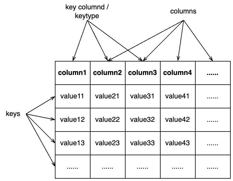
The GO.db package is built on top of a low-level infrastructure package AnnotationDbi. Thus, almost all Bioconductor “official data packages” inhert the same interface for querying data. Two important points:

There is a database object which has the same name as the package name.
They all implement the select() interface where the “database” can be thought of as a single virtual table.

GO.db

## GODb object:
## | GOSOURCENAME: 
## | GOSOURCEURL: 
## | GOSOURCEDATE: 
## | Db type: GODb
## | package: AnnotationDbi
## | DBSCHEMA: GO_DB
## | GOEGSOURCEDATE: 2024-Sep20
## | GOEGSOURCENAME: Entrez Gene
## | GOEGSOURCEURL: ftp://ftp.ncbi.nlm.nih.gov/gene/DATA
## | DBSCHEMAVERSION: 2.1

GO.db is a relatively simple database. The typical use is as:

select(GO.db, keys = c("GO:0000001", "GO:0000002"), columns = c("ONTOLOGY", "TERM"))

##         GOID ONTOLOGY                             TERM
## 1 GO:0000001       BP        mitochondrion inheritance
## 2 GO:0000002       BP mitochondrial genome maintenance

It can be read as “select records in the ONTOLOGY and TERM columns of the GO.db table where GOID is GO:0000001 or GO:0000002”.

The valid columns that can be searched in:

keytypes(GO.db)

## [1] "DEFINITION" "GOID"       "ONTOLOGY"   "TERM"

The valid columns that can be get value from.

columns(GO.db)

## [1] "DEFINITION" "GOID"       "ONTOLOGY"   "TERM"

In most cases keytypes() and columns() return the same set of columns.

Question: How to get all BP terms with select()?

select(GO.db, keys = "BP", keytype = "ONTOLOGY", columns = c("GOID", "TERM"))

Unfortunately, we cannot use select() to query something like: “select go_id from GO.db where the namespace is ‘BP’ and go_name contains ‘cell cycle’”. select() is not a full functional search interface of the internal SQLite database. You need to do it in two steps.

get the complete table of BP terms and save it as an R data frame.
filter the data frame in R

tb = select(GO.db, keys = "BP", keytype = "ONTOLOGY", columns = c("GOID", "TERM"))
tb[grep("cell cycle", tb$TERM), ] |> head()

##    ONTOLOGY       GOID                                                    TERM
## 26       BP GO:0000075                         cell cycle checkpoint signaling
## 31       BP GO:0000082                   G1/S transition of mitotic cell cycle
## 34       BP GO:0000086                   G2/M transition of mitotic cell cycle
## 76       BP GO:0000278                                      mitotic cell cycle
## 93       BP GO:0000320                        re-entry into mitotic cell cycle
## 94       BP GO:0000321 re-entry into mitotic cell cycle after pheromone arrest

The hierarchical relations of GO terms

GO.db provides variables that contain relations between GO terms. Taking biological process (BP) namespace as an example, there are the following four variables (similar for other two namespaces, but with GOCC and GOMF prefix).

GOBPCHILDREN
GOBPPARENTS
GOBPOFFSPRING
GOBPANCESTOR

GOBPCHILDREN and GOBPPARENTS contain parent-child relations. GOBPOFFSPRING contains all offspring terms of GO terms (i.e., all downstream terms of a term in the GO tree) and GOBPANCESTOR contains all ancestor terms of a GO term (i.e., all upstream terms of a term). The information in the four variables are actually redundant, e.g., GOBPOFFSPRING can be constructed from GOBPCHILDREN recursively. However, these pre-computated objects will save time in downstream analysis because traversing the GO tree is time-consuming.

The four variables are in the same format (objects of the AnnDbBimap class). Taking GOBPCHILDREN as an example, we can convert it to a simpler format by:

as.list()
asTable()

as.list() is also suggested by GO.db in its documentation.

lt = as.list(GOBPCHILDREN)
head(lt)

## $`GO:0000001`
## [1] NA
## 
## $`GO:0000002`
##      part of 
## "GO:0032042" 
## 
## $`GO:0000011`
## [1] NA
## 
## $`GO:0000012`
##            regulates negatively regulates positively regulates 
##         "GO:1903516"         "GO:1903517"         "GO:1903518" 
##                  isa                  isa 
##         "GO:1903823"         "GO:1990396" 
## 
## $`GO:0000017`
## [1] NA
## 
## $`GO:0000018`
##          isa          isa          isa          isa          isa          isa 
## "GO:0000019" "GO:0010520" "GO:0010569" "GO:0045191" "GO:0045910" "GO:0045911" 
##          isa          isa          isa 
## "GO:0061806" "GO:0072695" "GO:1903110"

lt is a simple list of vectors where each vector are child terms of a specific GO term, e.g., GO:0000002 has a child term GO:0032042. The element vectors in lt are also named and the names represent the relation of the child term to the parent term. When the element vector has a value NA, e.g. GO::0000001, this means the GO term is a leaf in the GO tree, and it has no child term (in this scenario, using character(0) instead of NA might be more proper).

toTable() converts the object to a data frame which provides identical information as the list:

tb = toTable(GOBPCHILDREN)
head(tb)

##        go_id      go_id     RelationshipType
## 1 GO:0032042 GO:0000002              part of
## 2 GO:1903516 GO:0000012            regulates
## 3 GO:1903517 GO:0000012 negatively regulates
## 4 GO:1903518 GO:0000012 positively regulates
## 5 GO:1903823 GO:0000012                  isa
## 6 GO:1990396 GO:0000012                  isa

Unfortunately, the first two columns in tb have the same name. A good idea is to add meaningful column names to it.

colnames(tb)[1:2] = c("child", "parent")

Please note, the previous column names c("child", "parent") are only valid for GOBPCHILDREN. If it is from one of the three GOBP* objects, readers please inspect the output to determine proper column names for it. E.g. you should assign c("parent", "child") to GOBPPARENTS.

With tb, we can calculate the fraction of different relations of GO terms.

tb = toTable(GOBPCHILDREN)
table(tb[, 3])

## 
##                  isa negatively regulates              part of 
##                46920                 2639                 4825 
## positively regulates            regulates 
##                 2650                 3040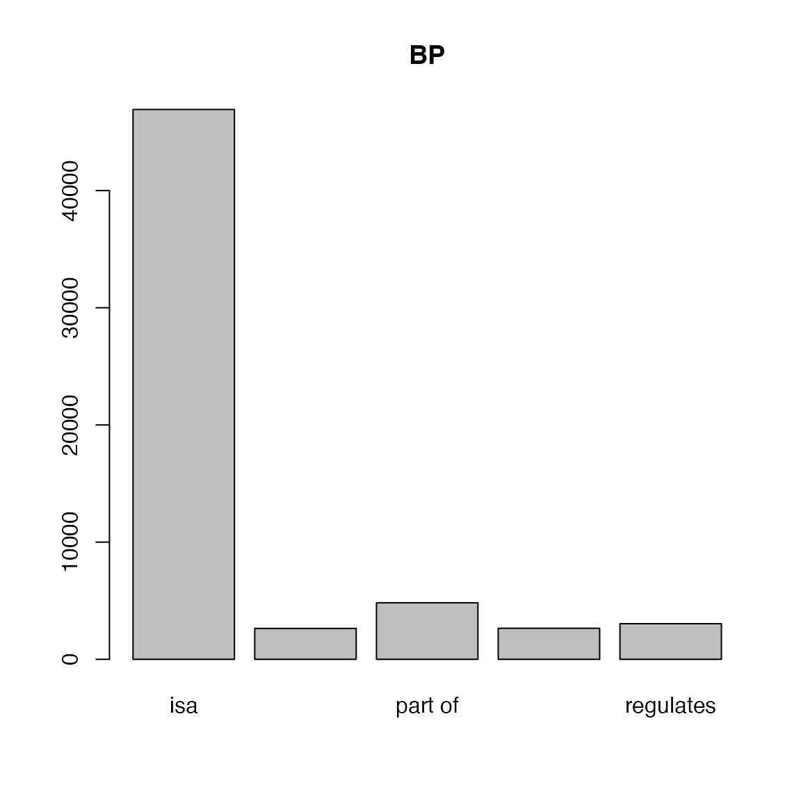

barplot(table(tb[, 3]), main = "BP")

tb = toTable(GOMFCHILDREN)
table(tb[, 3])

## 
##     isa part of 
##   12827       8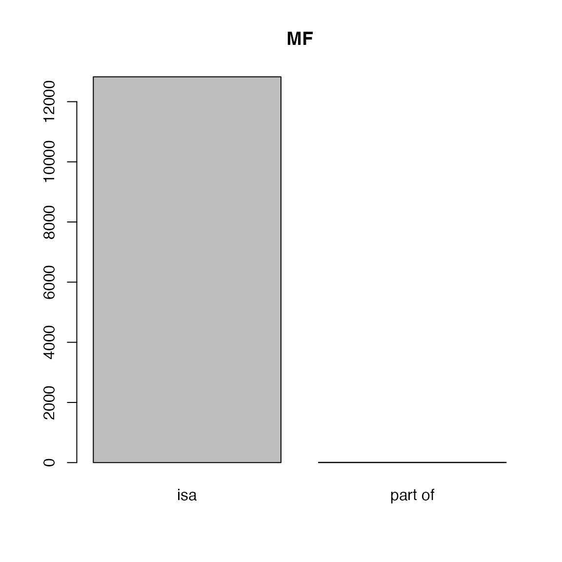

barplot(table(tb[, 3]), main = "MF")

tb = toTable(GOCCCHILDREN)
table(tb[, 3])

## 
##     isa part of 
##    4617    1787

barplot(table(tb[, 3]), main = "CC")

We can look at the distribution of the numbers of GO terms in each object.

Number of child terms. The following plot shows it follows a power-law distribution (majority of GO terms have very few child terms).

lt = as.list(GOBPCHILDREN)
tb = table(sapply(lt, length))
x = as.numeric(names(tb))
y = as.vector(tb)

library(ggplot2)
ggplot(data.frame(x = x, y = y), aes(x = x, y = y)) +
    geom_point() +
    scale_x_continuous(trans='log10') +
    scale_y_continuous(trans='log10') +
    labs(x = "Number of child terms", y = "Number of GO terms") + ggtitle("GOBPCHILDREN")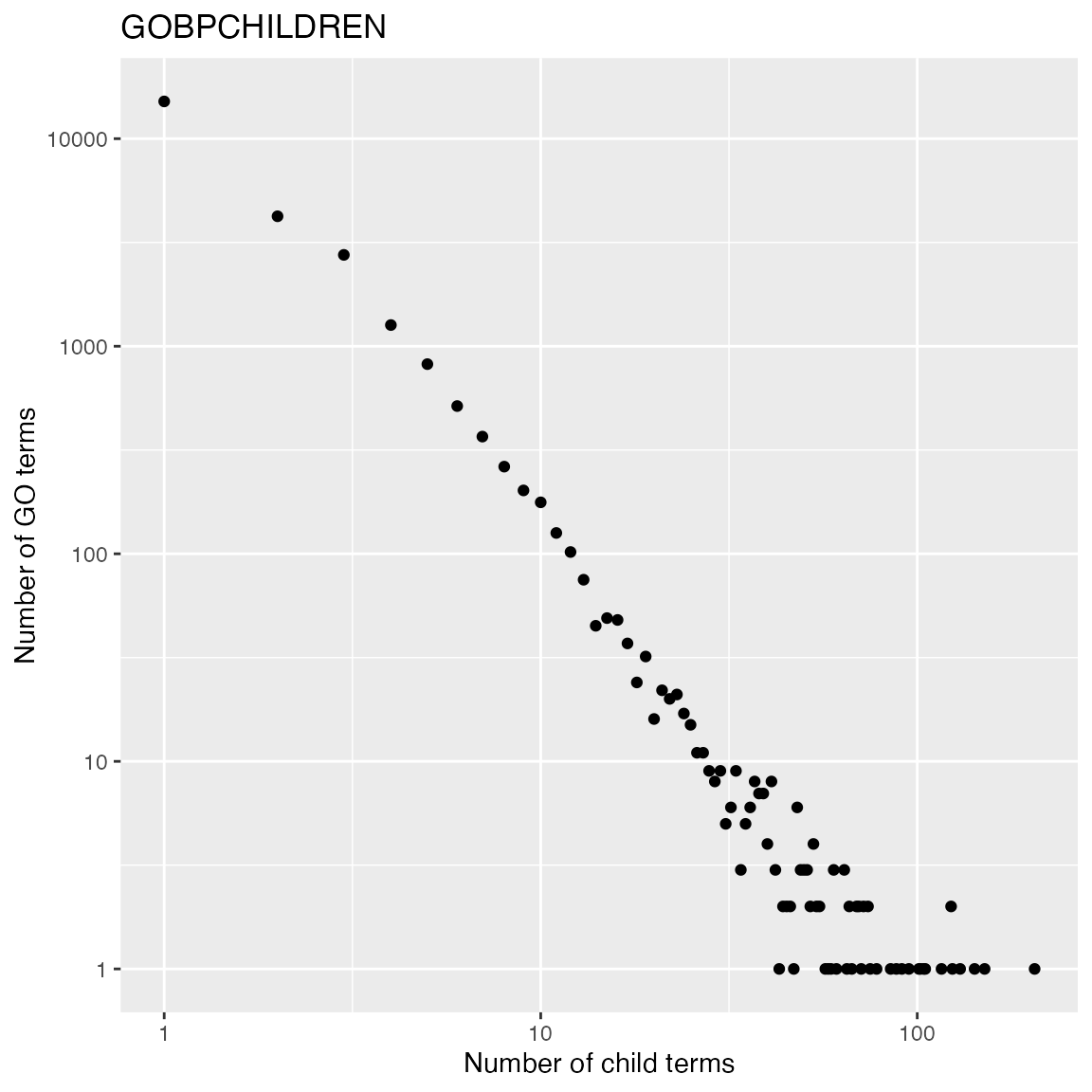

Number of parent terms. The term “GO:0008150” (biological process) is removed from the analysis because it is the top node in BP namespace and it has no parent term.

lt = as.list(GOBPPARENTS)
lt = lt[names(lt) != "GO:0008150"]
tb = table(sapply(lt, length))
x = as.numeric(names(tb))
y = as.vector(tb)

ggplot(data.frame(x = x, y = y), aes(x = x, y = y)) +
    geom_point() +
    scale_y_continuous(trans='log10') +
    labs(x = "Number of parent terms", y = "Number of GO terms") + ggtitle("GOBOPARENTS")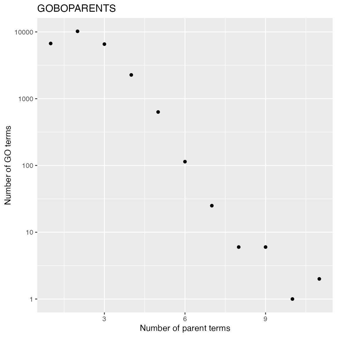

GOBPCHILDREN and GOBPPARENTS contain “local/direct” relations between GO terms, GOBPOFFSPRING and GOBPANCESTOR contain “local + distal” relations between GO terms.

lt = as.list(GOBPOFFSPRING)
lt[1:2]

## $`GO:0000001`
## [1] NA
## 
## $`GO:0000002`
##  [1] "GO:0006264" "GO:0032042" "GO:0032043" "GO:0043504" "GO:0090296"
##  [6] "GO:0090297" "GO:0090298" "GO:0110166" "GO:0140909" "GO:1901858"
## [11] "GO:1901859" "GO:1901860" "GO:1905951"

tb = toTable(GOBPOFFSPRING)
head(tb)

##        go_id      go_id
## 1 GO:0006264 GO:0000002
## 2 GO:0032042 GO:0000002
## 3 GO:0032043 GO:0000002
## 4 GO:0043504 GO:0000002
## 5 GO:0090296 GO:0000002
## 6 GO:0090297 GO:0000002

For querying single GO terms, you don’t need to explicitly convert the object to a list, but using [[ instead.

We can compare child terms and all offspring terms of “GO:0000002”:

GOBPCHILDREN[["GO:0000002"]]

##      part of 
## "GO:0032042"

GOBPOFFSPRING[["GO:0000002"]]

##  [1] "GO:0006264" "GO:0032042" "GO:0032043" "GO:0043504" "GO:0090296"
##  [6] "GO:0090297" "GO:0090298" "GO:0110166" "GO:0140909" "GO:1901858"
## [11] "GO:1901859" "GO:1901860" "GO:1905951"

There is a pseudo term in GO.db with the name “all”, which connects three ontologies of GO.

GOTERM[["all"]]

## GOID: all
## Term: all
## Ontology: universal
## Definition: NA

This all term is only recorded in GOBPPARENTS and GOBPANCESTOR.

GOBPPARENTS[["GO:0008150"]]

##   isa 
## "all"

There are several methods to construct GOBPOFFSPRING from GOBPCHILDREN/GOBPPARENTS.

For each term, we can recursively add child terms until reaching the leaf terms. This method traverses the GO DAG from top (root) to bottom (leaves) in a depth-first search manner.

lt_children = as.list(GOBPCHILDREN)

add_children = function(term, env) {
    children = lt_children[[term]]
    if(identical(children, NA)) {
        return(NULL)
    }
    env$offspring = c(env$offspring, children)
    lapply(children, add_children, env)
}

i = 0
lt_offspring = lapply(lt_children, function(x) {
    i <<- i + 1
    cat(i, "/", length(lt_children), "\n")
    if(identical(x, NA)) {
        return(x)
    } else {
        env = new.env()
        env$offspring = character(0)
        for(y in x) {
            add_children(y, env)
        }
        unique(env$offspring)
    }
})

This method is very slow due to that a term may have multiple parents. Then a parent-child relation may be repeated visited for terms close to root.

Or we traverse the DAG from bottom to top, and we recursively add the set of offsprings of a term to its parent terms. This method also sues GOBPPARENTS.

current_terms = names(lt_children)[sapply(lt_children, function(x) identical(x, NA))]
lt_offspring = vector("list", length(lt_children))
names(lt_offspring) = names(lt_children)
lt_parents = as.list(GOBPPARENTS)
while(length(current_terms)) {
    current_terms2 = NULL
    for(t in current_terms) {
        for(p in setdiff(lt_parents[[t]], "all")) {
            lt_offspring[[p]] = union(c(lt_offspring[[t]], t), lt_offspring[[p]])
            current_terms2 = c(current_terms2, p)
        }
    }
    current_terms = unique(current_terms2)
}
lt_offspring = lapply(lt_offspring, unique)

This method is more efficient because the parent-child relation is only visited once in the traversal.

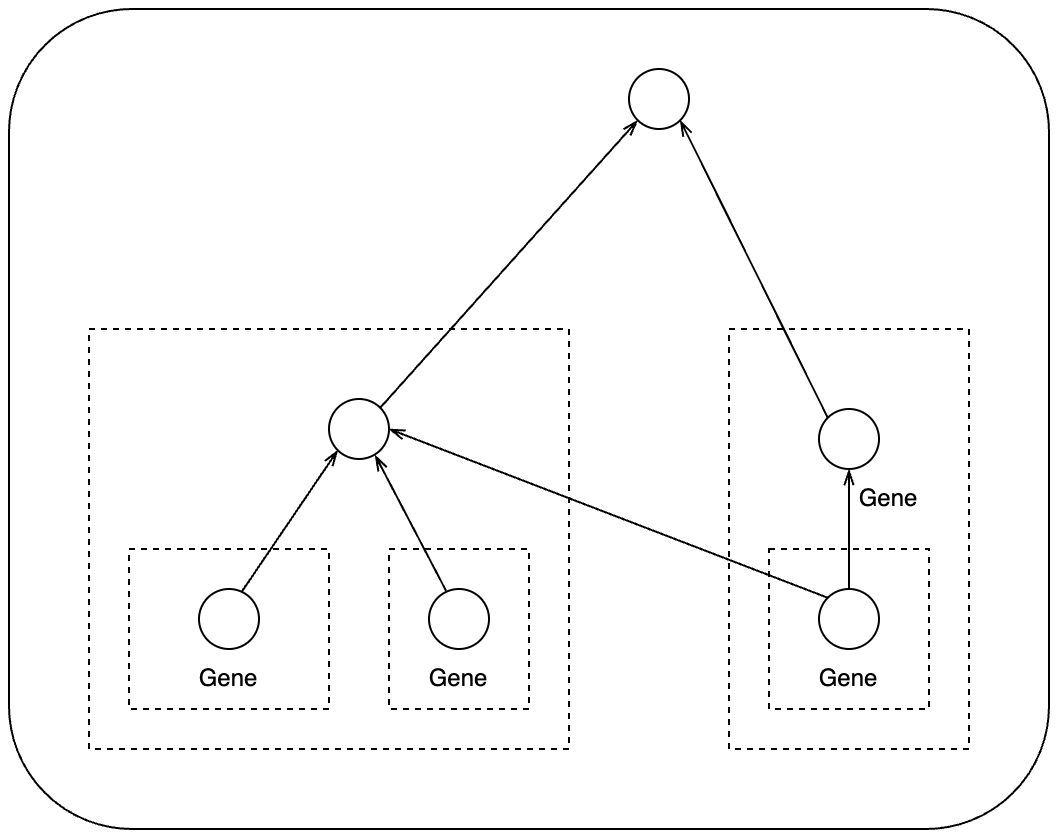
Link GO terms to genes

GO.db only contains information for GO terms. GO also provides gene annotated to GO terms, by manual curation or computational prediction. Such annotations are represented as mappings between GO IDs and gene IDs from external databases, which are usually synchronized between major public databases such as NCBI.

org.Hs.eg.db

To obtains genes in each GO term in R, Bioconductor provides a family of packages with name of org.*.db. Let’s take human for example, the corresponding package is org.Hs.eg.db. org.Hs.eg.db provides a standard way of providing mappings from Entrez gene IDs to a variaty of other databases.

library(org.Hs.eg.db)

Similarly, org.Hs.eg.db is a database object.

org.Hs.eg.db

## OrgDb object:
## | DBSCHEMAVERSION: 2.1
## | Db type: OrgDb
## | Supporting package: AnnotationDbi
## | DBSCHEMA: HUMAN_DB
## | ORGANISM: Homo sapiens
## | SPECIES: Human
## | EGSOURCEDATE: 2024-Sep20
## | EGSOURCENAME: Entrez Gene
## | EGSOURCEURL: ftp://ftp.ncbi.nlm.nih.gov/gene/DATA
## | CENTRALID: EG
## | TAXID: 9606
## | GOSOURCENAME: 
## | GOSOURCEURL: 
## | GOSOURCEDATE: 
## | GOEGSOURCEDATE: 2024-Sep20
## | GOEGSOURCENAME: Entrez Gene
## | GOEGSOURCEURL: ftp://ftp.ncbi.nlm.nih.gov/gene/DATA
## | KEGGSOURCENAME: KEGG GENOME
## | KEGGSOURCEURL: ftp://ftp.genome.jp/pub/kegg/genomes
## | KEGGSOURCEDATE: 2011-Mar15
## | GPSOURCENAME: UCSC Genome Bioinformatics (Homo sapiens)
## | GPSOURCEURL: ftp://hgdownload.cse.ucsc.edu/goldenPath/hg38/database
## | GPSOURCEDATE: 2024-Sep22
## | ENSOURCEDATE: 2024-May14
## | ENSOURCENAME: Ensembl
## | ENSOURCEURL: ftp://ftp.ensembl.org/pub/current_fasta
## | UPSOURCENAME: Uniprot
## | UPSOURCEURL: http://www.UniProt.org/
## | UPSOURCEDATE: Mon Sep 23 15:46:45 2024

You can use select() to obtain gene-GO term relations, but there are already objects calculated and easier to use. In this package, there are two objects for mapping between GO IDs and genes:

org.Hs.egGO2EG
org.Hs.egGO2ALLEGS

The difference between the two objects is org.Hs.egGO2EG contains genes that are directly annotated to every GO term, while org.Hs.egGO2ALLEGS contains genes that directly assigned to the GO term, as well as genes assigned to all its offspring terms. For example if term A is a parent of term B where A is more general, genes with function B should also have function A. Thus org.Hs.egGO2ALLEGS is the correct object for GO gene sets.

Again, org.Hs.egGO2ALLEGS is a vector-like object. There are two ways to obtain gene annotations to GO terms.

as.list()
toTable()

lt = as.list(org.Hs.egGO2ALLEGS)
lt[3:4]

## $`GO:0000017`
##    IDA    IMP    ISS    IDA 
## "6523" "6523" "6523" "6524" 
## 
## $`GO:0000018`
##         IDA         IDA         IDA         IDA         IEA         IMP 
##        "25"        "60"        "86"       "142"       "604"       "641" 
##         IDA         IEA         IEA         IDA         IDA         IDA 
##       "708"       "940"       "958"      "1111"      "1387"      "1457" 
##         IBA         IMP         IBA         IDA         IDA         IBA 
##      "2068"      "2074"      "2187"      "2521"      "2956"      "3005" 
##         IBA         IBA         IBA         IBA         IBA         IBA 
##      "3006"      "3007"      "3008"      "3009"      "3010"      "3024" 
##         IDA         IEA         ISS         TAS         TAS         NAS 
##      "3276"      "3558"      "3565"      "3565"      "3575"      "3586" 
##         TAS         TAS         IEA         TAS         IDA         IEA 
##      "3836"      "3838"      "4292"      "4361"      "4436"      "4436" 
##         ISS         IDA         ISS         IDA         IEA         IMP 
##      "4436"      "4437"      "4683"      "5347"      "5395"      "5531" 
##         IEA         IDA         IMP         IDA         IEA         ISS 
##      "5788"      "5888"      "6118"      "6502"      "6778"      "6830" 
##         IDA         IBA         IMP         ISS         IDA         IDA 
##      "6944"      "7014"      "7014"      "7014"      "7037"      "7040" 
##         IDA         IMP         ISS         IEA         IDA         IEA 
##      "7158"      "7158"      "7292"      "7320"      "7454"      "7468" 
##         IDA         IDA         IDA         IBA         IDA         IDA 
##      "8089"      "8295"      "8607"      "8741"      "8741"      "8914" 
##         IBA         IDA         IEA         IEA         IDA         ISS 
##      "8971"      "9025"      "9400"      "9466"      "9643"     "10039" 
##         IDA         IDA         IDA         IDA         IDA         IDA 
##     "10097"     "10111"     "10459"     "10524"     "10635"     "10721" 
##         IMP         IDA         IDA         IDA         IBA         IBA 
##     "10721"     "10856"     "10902"     "10933"     "11105"     "22891" 
##         IMP         IEA         ISS         IMP         IMP         IDA 
##     "22891"     "22976"     "22976"     "23028"     "23347"     "23514" 
##         ISS         IDA         IDA         IDA         IEA         IEA 
##     "23529"     "26122"     "26168"     "29072"     "30009"     "50943" 
##         IEA         ISS         IMP         IDA         IDA         IBA 
##     "51010"     "51111"     "51149"     "51548"     "51588"     "51750" 
##         IMP         ISS         ISS         IBA         IDA         IDA 
##     "51750"     "51750"     "54386"     "54537"     "54537"     "54556" 
##         IDA         IBA         IMP         ISS         IDA         IDA 
##     "54799"     "55010"     "55010"     "55063"     "55086"     "55135" 
##         IDA         ISS         IDA         IDA         IDA         IBA 
##     "55183"     "55183"     "55257"     "55658"     "55929"     "56154" 
##         IDA         IEP         ISS         IBA         IMP         IDA 
##     "56893"     "56916"     "56941"     "56979"     "56979"     "57162" 
##         IDA         IDA         IDA         IDA         IDA         IEA 
##     "57599"     "57634"     "63979"     "64110"     "64769"     "79915" 
##         IDA         IDA         IEA         IDA         IMP         ISS 
##     "80311"     "80314"     "80762"     "84083"     "84717"     "84787" 
##         IDA         IBA         IMP         ISS         IBA         IDA 
##     "84893"     "92797"     "92797"    "113510"    "115004"    "115004" 
##         IBA         IEA         ISS         IEA         IBA         IBA 
##    "116028"    "118460"    "121260"    "126549"    "132243"    "149840" 
##         IDA         IMP         IMP         ISS         IMP         IMP 
##    "149840"    "151987"    "154288"    "154288"    "158880"    "196528" 
##         IEA         ISS         IBA         IBA         IDA         ISS 
##    "200558"    "201516"    "341567"    "373861"    "387893"    "441161" 
##         IBA         IDA 
## "112441434" "112441434"

If we compare to org.Hs.egGO2EG which contains incomplete genes:

lt2 = as.list(org.Hs.egGO2EG)
lt2[3:4]

## $`GO:0000017`
##    IDA    IMP    ISS    IDA 
## "6523" "6523" "6523" "6524" 
## 
## $`GO:0000018`
##     TAS     TAS     TAS     IEP 
##  "3575"  "3836"  "3838" "56916"

The gene IDs have names. They are evidence codes of how genes are annotated to GO terms.

Let’s try toTable():

tb = toTable(org.Hs.egGO2ALLEGS)
head(tb)

##   gene_id      go_id Evidence Ontology
## 1       1 GO:0002376      IBA       BP
## 2       1 GO:0002682      IBA       BP
## 3       1 GO:0002764      IBA       BP
## 4       1 GO:0006955      IBA       BP
## 5       1 GO:0007154      IBA       BP
## 6       1 GO:0007165      IBA       BP

Now there is an additional column "Ontology". This is convinient because org.Hs.egGO2ALLEGS contains GO terms from the three namespaces and the as.list() cannot distinguish the different namespaces.

tb[tb$Ontology == "BP", ]

onto = Ontology(GOTERM)
lt[ onto(names(lt)) == "BP" ]

Let’s calculate the frequency of evidence code:

barplot(sort(table(tb$Evidence)))

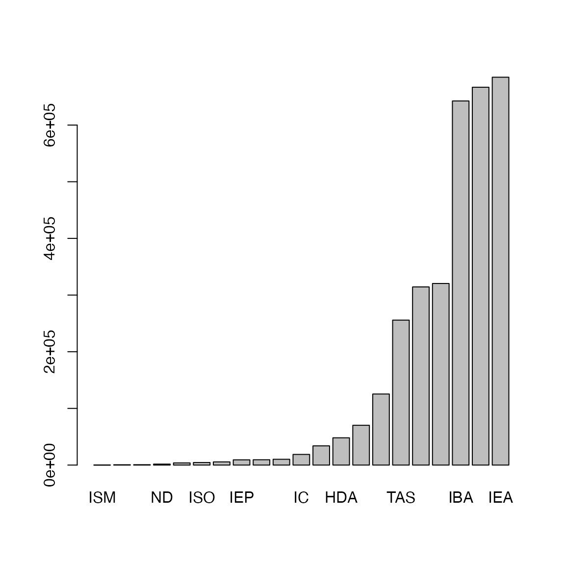
Now it seems we have obtained the complete gene-GO relations. Can we directly use org.Hs.egGO2ALLEGS as the GO gene sets? The answer is no, check the gene annotation for “GO:0000002”:

org.Hs.egGO2ALLEGS[["GO:0000002"]]

##      IMP      TAS      IDA      IMP      IMP      IMP      ISS      IBA 
##    "142"    "291"   "1763"   "1890"   "2021"   "3980"   "4205"   "4358" 
##      IMP      IMP      IBA      IDA      IMP      IMP      IBA      IDA 
##   "4358"   "4976"   "5428"   "5428"   "5428"   "6240"   "6742"   "6742" 
##      IMP      IEA      IEA      NAS      IMP      IBA       IC      IDA 
##   "7156"   "7157"   "9093"   "9361"  "10000"  "11232"  "11232"  "11232" 
##      IMP      IBA      IDA      IBA      IMP      NAS      IMP      IEA 
##  "50484"  "55186"  "55186"  "56652"  "56652"  "56652"  "64863"  "80119" 
##      IEA      IBA      IDA      IEA      IBA      IMP      TAS      IEA 
##  "83667"  "84275"  "84275"  "84461"  "92667"  "92667"  "92667" "131474" 
##      IBA      IMP      ISS      IMP 
## "201973" "201973" "201973" "219736"

A gene can be duplicatedly annotated to a GO term with different evidence code. Thus, to obtain the GO gene sets, we need to take the unique genes.

Let’s compare gene duplications in GO gene sets:

n1 = sapply(lt, length)
lt = lapply(lt, unique)
n2 = sapply(lt, length)

plot(n1, n2, xlim = c(0, max(n1)), ylim = c(0, max(n1)),
    xlab = "with duplicated", ylab = "without duplicated",
    main = "number of genes in GO BP gene sets")

With tb, we can look at the distribution of numbers of genes in GO gene sets. It approximately follows a power-law distribution. This means majority of GO gene sets only contain intermediate numbers of genes.

Let’s compare gene duplications in GO gene sets:

tb = toTable(org.Hs.egGO2ALLEGS)
tb = unique(tb[tb$Ontology == "BP", 1:2])
t1 = table(table(tb$go_id))
x1 = as.numeric(names(t1))
y1 = as.vector(t1)
ggplot(data.frame(x = x1, y = y1), aes(x = x, y = y)) +
    geom_point() +
    scale_x_continuous(trans='log10') +
    scale_y_continuous(trans='log10') +
    labs(x = "Number of annotated genes", y = "Number of GO terms") + ggtitle("GOBP")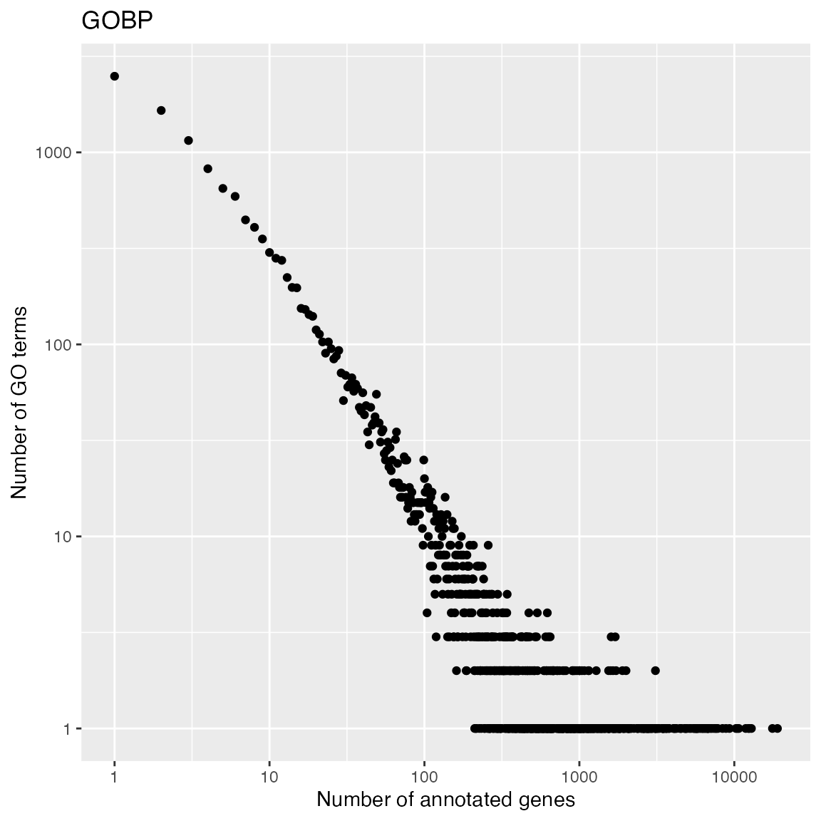

And the distribution of numbers of GO gene sets that a gene is annotated.

t2 = table(table(tb$gene_id))
x2 = as.numeric(names(t2))
y2 = as.vector(t2)
ggplot(data.frame(x = x2, y = y2), aes(x = x, y = y)) +
    geom_point() +
    scale_x_continuous(trans='log10') +
    scale_y_continuous(trans='log10') +
    labs(x = "Number of gene sets", y = "Number of genes") + ggtitle("GOBP")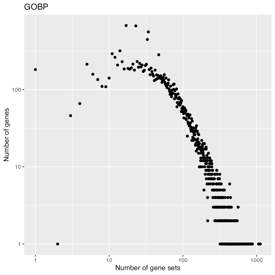

Biocondutor core team maintains org.*.db for 18 organisms

Package	Organism	Package	Organism
`org.Hs.eg.db`	Human	`org.Ss.eg.db`	Pig
`org.Mm.eg.db`	Mouse	`org.Gg.eg.db`	Chicken
`org.Rn.eg.db`	Rat	`org.Mmu.eg.db`	Rhesus monkey
`org.Dm.eg.db`	Fruit fly	`org.Cf.eg.db`	Canine
`org.At.tair.db`	Arabidopsis	`org.EcK12.eg.db`	E coli strain K12
`org.Sc.sgd.db`	Yeast	`org.Xl.eg.db`	African clawed frog
`org.Dr.eg.db`	Zebrafish	`org.Ag.eg.db`	Malaria mosquito
`org.Ce.eg.db`	Nematode	`org.Pt.eg.db`	Chimpanzee
`org.Bt.eg.db`	Bovine	`org.EcSakai.eg.db`	E coli strain Sakai

Use the `select()` interface

This is normally a two-step process:

get all genes
get all GO terms

because org.Hs.eg.db is thought of to provide ID mappings between databases.

all_genes = keys(org.Hs.eg.db, keytype = "ENTREZID")
tb = select(org.Hs.eg.db, keys = all_genes, keytype = "ENTREZID", 
    columns = c("GOALL", "ONTOLOGYALL"))
head(tb)

##   ENTREZID      GOALL EVIDENCEALL ONTOLOGYALL
## 1        1 GO:0002376         IBA          BP
## 2        1 GO:0002682         IBA          BP
## 3        1 GO:0002764         IBA          BP
## 4        1 GO:0003674          ND          MF
## 5        1 GO:0005575         HDA          CC
## 6        1 GO:0005575         IBA          CC

Then you might need to take the unique genes:

tb = tb[tb$ONTOLOGYALL == "BP", 1:2]
tb = unique(tb)
head(tb)

##    ENTREZID      GOALL
## 1         1 GO:0002376
## 2         1 GO:0002682
## 3         1 GO:0002764
## 16        1 GO:0006955
## 17        1 GO:0007154
## 18        1 GO:0007165

Note the column ONTOLOGYALL can also be a valid “keytype” column, then actually we can do “select all genes and GO terms where ontology is BP”:

tb = select(org.Hs.eg.db, keys = "BP", keytype = "ONTOLOGYALL", columns = c("ENTREZID", "GOALL"))
# and remember to remove duplicated genes

Pay attention you should always use the columns with suffix “ALL” in the names for getting complete GO gene sets.

Practice

Practice 1

We have demonstrated a gene can be duplicatedly annotated to a same GO term. Taking org.Hs.egGO2ALLEGS, can you calculate the percent of GO terms that have duplicated genes?

lt = as.list(org.Hs.egGO2ALLEGS)
n = length(lt)
nd = sum(sapply(lt, function(x) any(duplicated(x))))
nd/n

## [1] 0.5368885

Practice 2

org.Hs.egGO2ALLEGS has already merged genes annotated to all offspring terms. Try to manually construct GO gene sets with GOBPOFFSPRING and org.Hs.egGO2EGS, then compare to gene sets in org.Hs.egGO2ALLEGS.

lt_genes = as.list(org.Hs.egGO2EG)
lt_terms = as.list(GOBPOFFSPRING)

For a GO term, we need to consider its offspring terms + the term itself:

for(nm in names(lt_terms)) {
    lt_terms[[nm]] = c(lt_terms[[nm]], nm)
}

Merge annotated genes for all offspring terms:

lt_genes_manual = lapply(lt_terms, function(x) {
    unique(unlist(lt_genes[x]))
})

Compare to org.Hs.egGO2ALLEGS:

lt_genes_all = as.list(org.Hs.egGO2ALLEGS)
lt_genes_all = lapply(lt_genes_all, unique)

cn = intersect(names(lt_genes_manual), names(lt_genes_all))
plot(sapply(lt_genes_manual[cn], length), sapply(lt_genes_all[cn], length), log = "xy",
    xlab = "manual gene sets", ylab = "org.Hs.egGO2ALLEGS")

Zuguang Gu z.gu@dkfz.de

2025-05-31

The GO.db package

As a vector-object

As a table-object

The hierarchical relations of GO terms

Link GO terms to genes

org.Hs.eg.db

Use the `select()` interface

Practice

Practice 1

Practice 2

Topic 1-01: GO gene sets

Zuguang Gu z.gu@dkfz.de

2025-05-31

The GO.db package

As a vector-object

As a table-object

The hierarchical relations of GO terms

Link GO terms to genes

org.Hs.eg.db

Use the select() interface

Practice

Practice 1

Practice 2

Use the `select()` interface