Topic 2-05: fgsea
Zuguang Gu z.gu@dkfz.de
2025-05-31
Source:vignettes/topic2_04_fgsea.Rmd
topic2_04_fgsea.RmdThe permutation-based method is by nature very slow, especially if you want to get p-values in high precision. In this document, we demonstrate the use of an extremely fast package fgsea, but only for the gene-permutation-based method.
We still use the p53 dataset.
library(GSEAtopics)
data(p53_dataset)
s = p53_dataset$s
gs = p53_dataset$gs
The use of fgsea is striaghtforward. Just use the
fgsea() function:
##                            pathway      pval      padj    log2err         ES
##                             <char>     <num>     <num>      <num>      <num>
## 1:                     41bbPathway 0.5826772 0.8437021 0.08553569  0.2709496
## 2: ADULT_LIVER_vs_FETAL_LIVER_GNF2 0.4524457 0.7673679 0.06464846 -0.2593511
## 3:     ANDROGEN_GENES_FROM_NETAFFX 0.5583333 0.8348651 0.05571042 -0.2476218
## 4:               ANDROGEN_UP_GENES 0.0732458 0.4163595 0.28780513  0.2987018
## 5:                  ANTI_CD44_DOWN 0.7672634 0.9132431 0.06977925  0.2597386
## 6:                    ANTI_CD44_UP 0.6135338 0.8518277 0.05502111 -0.2848141
##           NES  size  leadingEdge
##         <num> <int>       <list>
## 1:  0.9004369    18 RELA, MA....
## 2: -1.0054655    61 RODH-4, ....
## 3: -0.9360798    53 RODH-4, ....
## 4:  1.3105071    57 VAPA, LM....
## 5:  0.7597468    12 LAMP2, E....
## 6: -0.8918719    23 IL1A, AL....
You only need to make gene IDs in s (the names of the
vector) are the same as in gs.
Implement helper functions
The same as the ora_*() functions for different types of
gene sets, we can also implement the fgsea_*()
functions.
We first define a wrapper function where we rename the colnames of
the data frame from fgsea(), just let it be consistent to
the results from ora_*() functions. We also reorder the
result data frame by p-values.
fgsea_wrapper = function(s, gs, min_size = 5, max_size = 1000, ...) {
    s = sort(s, decreasing = TRUE)
    df = fgsea(gs, s, minSize = min_size, maxSize = max_size, ...)
    df = as.data.frame(df)
    colnames(df) = c("gene_set", "p_value", "p_adjust", "log2_p_err", "es", "nes", "n_gs", "leading_edge")
    df = df[order(df$p_value), , drop = FALSE]
    rownames(df) = NULL
    df
}
Now we can implement these helper functions. The logic is the same as
ora_*() functions. We first retrieve gene sets than apply
fgsea_wrapper().
fgsea_go = function(s, org_db = org.Hs.eg.db::org.Hs.eg.db, ontology = "BP") {
    tb = AnnotationDbi::select(org_db, keys = ontology, keytype = "ONTOLOGYALL",
        columns = c("ENTREZID", "GOALL"))
    gs = split(tb$ENTREZID, tb$GOALL)
    gs = lapply(gs, function(x) {
        as.character(unique(x))
    })

    fgsea_wrapper(s, gs)
}

fgsea_kegg = function(s, organism = "hsa") {
    pathway_genes = read.table(url(paste0("https://rest.kegg.jp/link/pathway/", organism)),
        sep = "\t", quote = "")
    pathway_genes[, 1] = gsub("^\\w+:", "", pathway_genes[, 1])
    pathway_genes[, 2] = gsub("^\\w+:", "", pathway_genes[, 2])
    pathway_genes = split(pathway_genes[, 1], pathway_genes[, 2])

    fgsea_wrapper(s, pathway_genes)
}
All these fgsea_*() functions use EntreZ IDs as the
internal IDs. Then for the input gene score vector, genes should also
have EntreZ IDs.
Note, all fgsea_*() and fgsea::fgsea() do
not require s to be pre-sorted. It is sorted
internally.
Convert gene IDs
We have demonstrated how to convert gene IDs for a vector of genes. Here the scenario is a little bit different. Gene IDs are names of a numeric vevtor.
We first generate a global mapping between symbols and EntreZ IDs:
library(org.Hs.eg.db)
map = map_to_entrez("SYMBOL", org.Hs.eg.db)
map_to_entrez() only returns mapping for protein-coding
genes. According to the pratice we have made, the human, the mapping
between symbols and EntreZ IDs is one-to-one. But we need to be careful.
1. gene symbols change from time to time. You cannot ensure the symbol
used in the dataset is the most recent version. 2. for other organisms,
we don’t know whether the mapping is also one-to-one. Let’s do it in a
conservative way.
symbol = names(s)
entrez = map[symbol]
in entrez, there are possible NA values or
duplicated values. We first remove NAs:
s2 = unname(s) # since s2 will have EntreZ IDs as names
l = !is.na(entrez)
s2 = s2[l]
entrez = entrez[l]
Then remove duplicates, either only keep the first one, or take the mean.
I use the mean:
s2 = tapply(s2, entrez, mean)In GSEAtopics, there is a helper function
convert_to_entrez() which works on gene ID vecotr, numeric
vector with gene IDs as names, and matrix with gene IDs as row
names.
s2 = convert_to_entrez(s) # if is human, the the second argument can be omitted## gene id might be SYMBOL (p = 0.680 )And let’s try these fgsea_*() helper functions:
##     gene_set      p_value     p_adjust log2_p_err         es       nes n_gs
## 1 GO:0007186 2.081795e-10 1.524707e-06  0.8266573 -0.3600615 -1.838127  512
## 2 GO:0002682 1.783344e-08 6.530605e-05  0.7337620 -0.2997243 -1.581012  912
## 3 GO:0022402 3.322465e-07 8.111244e-04  0.6749629  0.2522013  1.540379  577
## 4 GO:0050776 2.609926e-06 4.547958e-03  0.6272567 -0.3066230 -1.570486  542
## 5 GO:0002684 3.104832e-06 4.547958e-03  0.6272567 -0.2981775 -1.543817  645
## 6 GO:1902850 4.695924e-06 5.732158e-03  0.6105269  0.4574162  2.065071   71
##   leading_edge
## 1 23620, 2....
## 2 1026, 58....
## 3 29899, 1....
## 4 581, 677....
## 5 1026, 58....
## 6 29899, 9....
head(fgsea_kegg(s2))## gene_set p_value p_adjust log2_p_err es nes n_gs
## 1 hsa04080 4.597341e-08 1.622861e-05 0.7195128 -0.4052099 -1.925672 234
## 2 hsa03010 1.335615e-07 2.357360e-05 0.6901325 -0.5122149 -2.131406 85
## 3 hsa04060 2.114913e-06 2.488548e-04 0.6272567 -0.3936669 -1.836075 193
## 4 hsa04940 1.209843e-05 1.067686e-03 0.5933255 -0.5971851 -2.141821 36
## 5 hsa04081 5.328841e-05 3.762162e-03 0.5573322 -0.3766489 -1.741364 180
## 6 hsa05332 8.980278e-05 5.283397e-03 0.5384341 -0.6071862 -2.068430 29
## leading_edge
## 1 23620, 2....
## 2 6223, 61....
## 3 355, 343....
## 4 355, 355....
## 5 2100, 15....
## 6 355, 355....In GSEAtopics there are the following
fgsea_*() functions:
Compare to the native implementations
Let’s have a quick comparison between the fgsea()
function and gene-permutation-based function we have implemented in the
previous document. We use the gsea_gene_perm() function
from the GSEAtopics package. Under the default setting,
both functions use the same statistic and perform two-sided test:
df1 = fgsea_wrapper(s, gs)
df2 = gsea_gene_perm(s, gs, verbose = FALSE)
We compare p-values and NES from the functions:
rownames(df1) = df1$gene_set
rownames(df2) = df2$gene_set

cn = intersect(rownames(df1), rownames(df2))
par(mfrow = c(1, 2))
plot(df1[cn, "p_value"], df2[cn, "p_value"], main = "p_value", xlab = "fgsea", ylab = "native")
plot(df1[cn, "nes"], df2[cn, "nes"], main = "nes", xlab = "fgsea", ylab = "native")
And for the one-sided test which only look for enrichment of up-regulated genes:
df1 = fgsea_wrapper(s, gs, scoreType = "pos")
df2 = gsea_gene_perm(s, gs, direction = "pos", verbose = FALSE)

rownames(df1) = df1$gene_set
rownames(df2) = df2$gene_set

cn = intersect(rownames(df1), rownames(df2))
par(mfrow = c(1, 2))
plot(df1[cn, "p_value"], df2[cn, "p_value"], main = "p_value", xlab = "fgsea", ylab = "native")
plot(df1[cn, "nes"], df2[cn, "nes"], main = "nes", xlab = "fgsea", ylab = "native")
Other ways to capture bi-directional changes
The default behavior of two-sided fgsea() or the GSEA
method is to capture the stronger one of the up- and down-regulation of
genes in a gene set. There are two other ways:
- If you want to keep enrichment for both up-regulated and down-regulated genes. You can perform two GSEA analysis, a one-sided test only for up-regulated genes and a second one-sided test only for down-regulated genes.
- if the gene score is log2fc-like, i.e. with both positive and
negative values, and if you do not care the direction of the
differential expression, you can use
|s|as the gene scores.
Which type of gene scores to use
GSEA requires a pre-calculated vector of gene-level scores. In the previous example, we use the signal-to-noise ratio. As there are many other ways to calculate a gene-level score. We ask, do they all perform similarly or which ones are better and which ones are worse?
Let’s go back to the original dataset, the matrix and the condition vector:
expr = p53_dataset$expr
condition = p53_dataset$condition
We try the following five metrics: log2 fold change, signal-to-noise ratio, t-value, -log p-value multiplies by the sign of t-values, SAM moderated t-value.
# from here, we use MUT as the treatment group
m1 = expr[, condition == "MUT"]
m2 = expr[, condition == "WT"]

library(matrixStats)
log2fc = log2(rowMeans(m1)/rowMeans(m2))
s2n = (rowMeans(m1) - rowMeans(m2))/(rowSds(m1) + rowSds(m2))

library(genefilter)
tdf = rowttests(expr, condition)  # equal variance
t_value = tdf$statistic
names(t_value) = rownames(tdf)
log_p = -log10(tdf$p.value)*sign(tdf$statistic)
names(log_p) = rownames(tdf)

n1 = ncol(m1)
n2 = ncol(m2)
v1 = rowVars(m1)
v2 = rowVars(m2)
sp = sqrt( ((n1-1)*v1 + (n2-1)*v2)/(n1 + n2 - 2) )*sqrt(1/n1 + 1/n2)
sam = (rowMeans(m1) - rowMeans(m2))/(sp + quantile(sp, 0.1))
First we can make a pairwise scatter plot to see the similarities of the five metrics:
pairs(data.frame(log2fc = log2fc, s2n = s2n, t_value = t_value, log_p = log_p, sam = sam), pch = ".")
We also look at the distribution of the five metrics:
par(mfrow = c(2, 3))
plot(sort(log2fc, decreasing = TRUE), main = "log2fc")
plot(sort(s2n, decreasing = TRUE), main = "s2n")
plot(sort(t_value, decreasing = TRUE), main = "t_value")
plot(sort(log_p, decreasing = TRUE), main = "log_p")
plot(sort(sam, decreasing = TRUE), main = "sam")
And we perform GSEA with five gene score vectors.
tb_log2fc  = fgsea_wrapper(sort(log2fc, decreasing = TRUE), gs)
tb_s2n     = fgsea_wrapper(sort(s2n, decreasing = TRUE), gs)
tb_t_value = fgsea_wrapper(sort(t_value, decreasing = TRUE), gs)
tb_log_p   = fgsea_wrapper(sort(log_p, decreasing = TRUE), gs)
tb_sam     = fgsea_wrapper(sort(sam, decreasing = TRUE), gs)
Top 50 most significant gene sets:
library(eulerr)
plot(euler(list(log2fc = tb_log2fc$gene_set[1:50],
                s2n = tb_s2n$gene_set[1:50],
                t_value = tb_t_value$gene_set[1:50],
                log_p = tb_log_p$gene_set[1:50],
                sam = tb_sam$gene_set[1:50])),
    quantities = TRUE)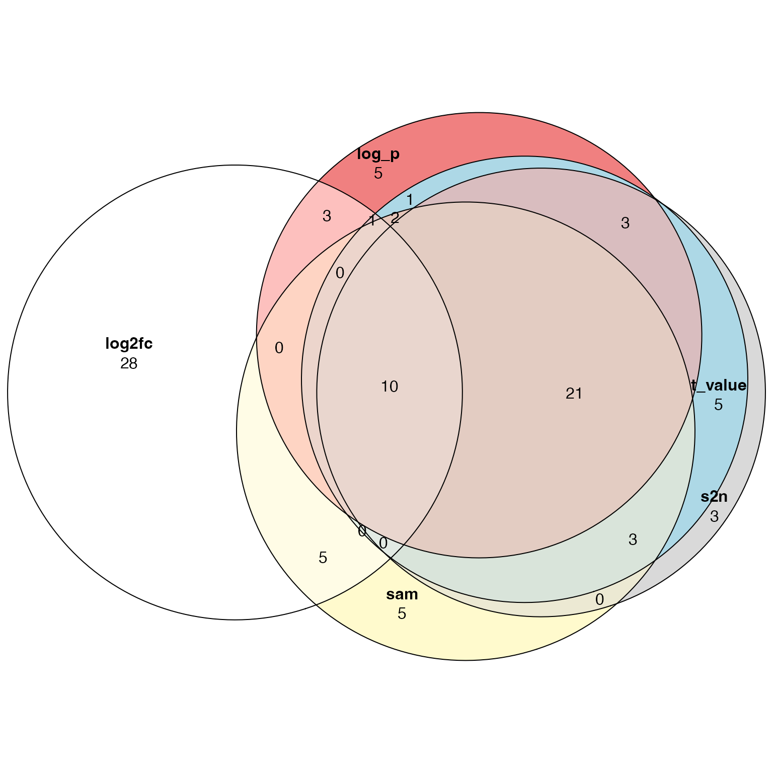
Conclusion: use t-value or similar metrics as gene-level scores for GSEA analysis. Log2fc is not recommended to use.