Topic 6-02: Cluster and summarize

Zuguang Gu z.gu@dkfz.de

2025-05-31

There are two types of similarity methods, the count-based and semantic-based. We look at them separately.

Count-based similarity

As an example, we use significant gene sets from ORA on the p53 dataset.

library(GSEAtopics)
data(p53_dataset)
expr = p53_dataset$expr
condition = p53_dataset$condition
gs = p53_dataset$gs

library(genefilter)
tdf = rowttests(expr, factor(condition))
diff = rownames(expr)[abs(tdf$statistic) > 2]
tb_ora = ora(diff, gs, universe = rownames(expr))
sig = tb_ora$gene_set[tb_ora$p_value < 0.05]

We suggest to only use the significant genes when calculating the similarities.

gs2 = lapply(gs[sig], function(x) intersect(x, diff))

Additionally adding the gene weight can sometimes improve the similarity patterns.

w = tdf$statistic
names(w) = rownames(tdf)

sm = jaccard(gs2, weight = abs(w))
diag(sm) = NA
library(ComplexHeatmap)
Heatmap(sm, name = "jaccard", col = c("white", "red"))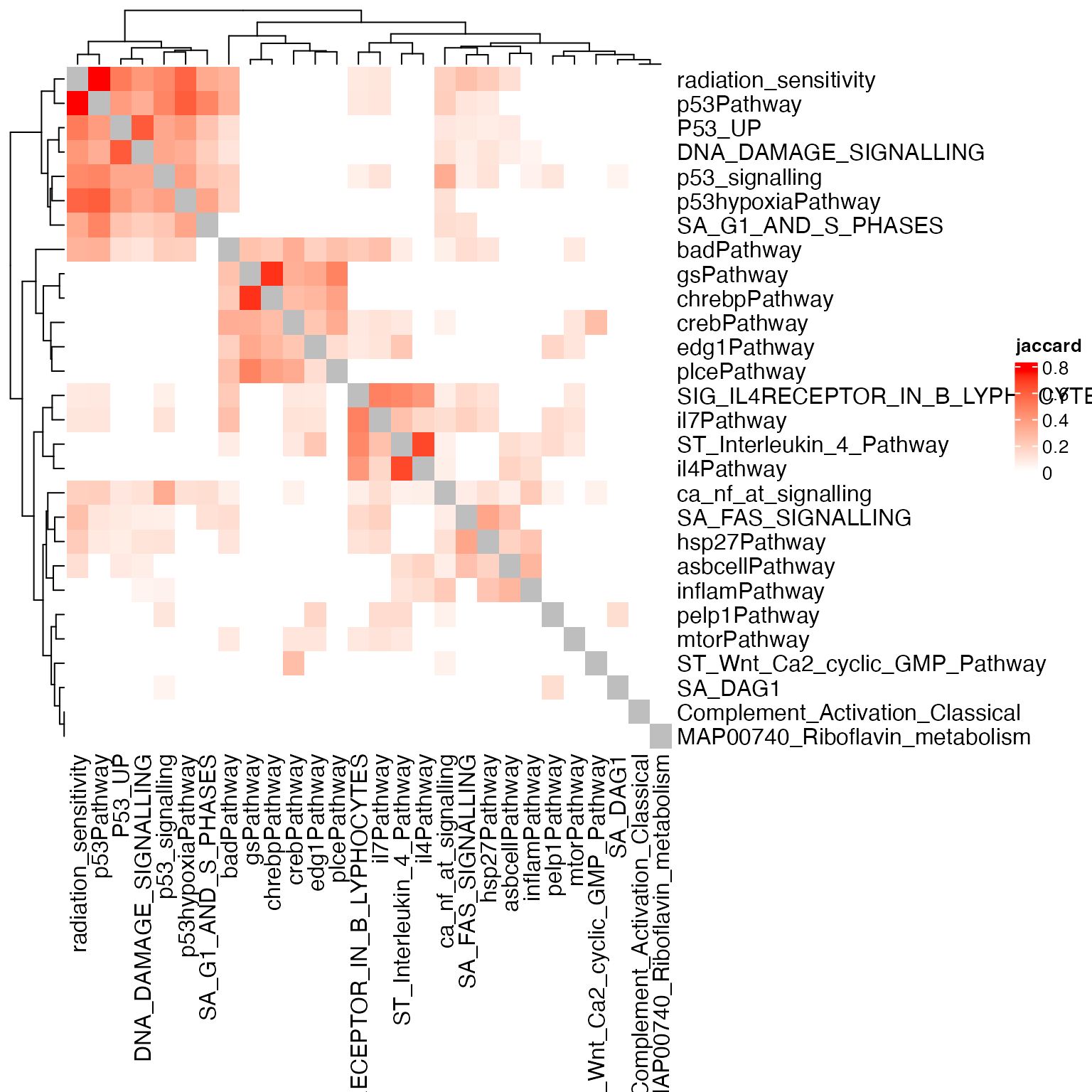

The block-pattern is very obvious. We can split it by hierarchical clustering + cutree, kmeans or any clustering methods. We recommend to use the graph-based clustering methods.

The similarity matrix can be thought of as an adjacency matrix. The igraph package provides many graph-based clustering methods.

library(igraph)
g = graph_from_adjacency_matrix(sm, weighted = TRUE, mode = "upper", diag = FALSE)
cl = membership(cluster_louvain(g))
Heatmap(sm, , name = "jaccard", col = c("white", "red"), border = "black",
    row_split = cl, column_split = cl)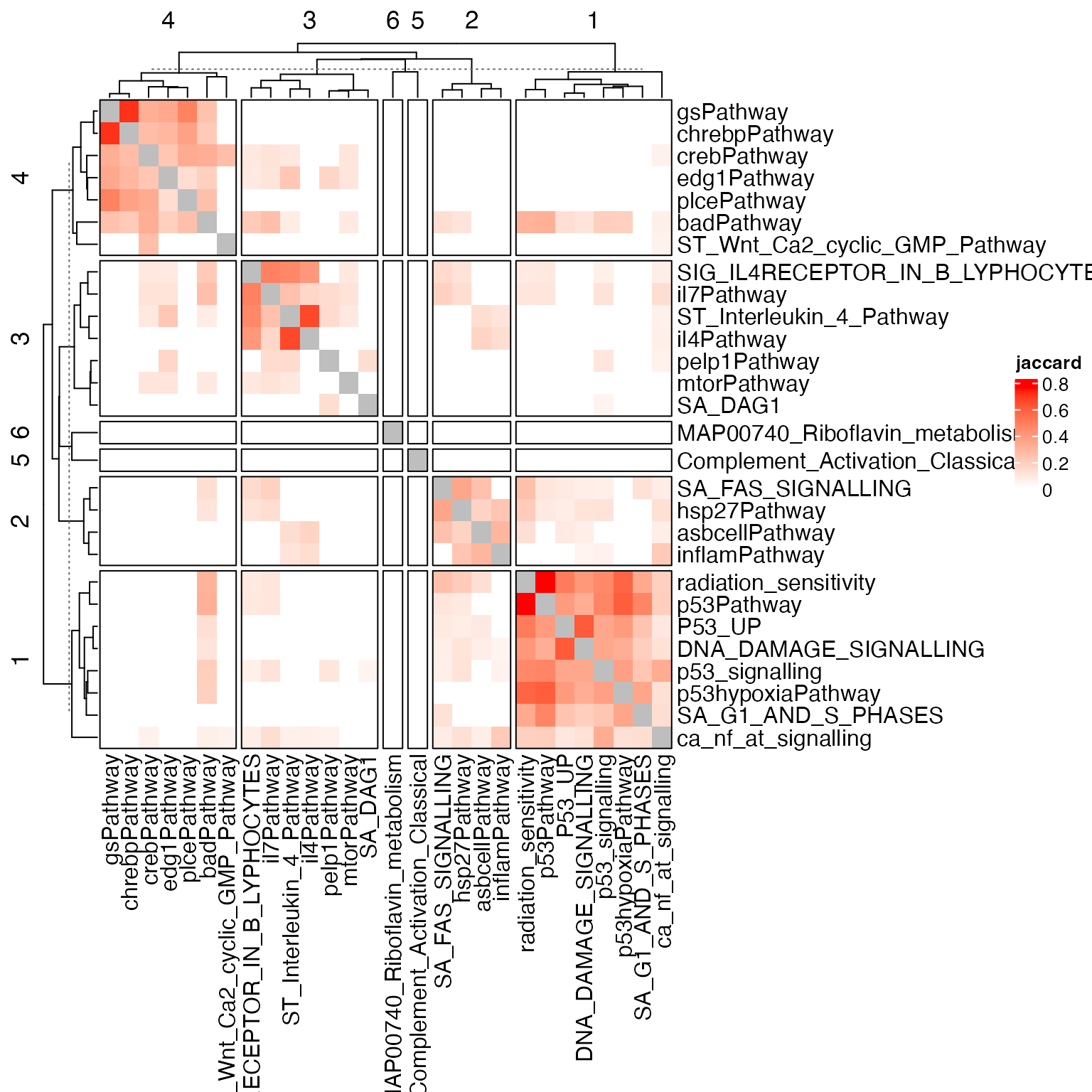

Clustering the gene sets is fairly easy. However, this is not the end of the analysis. We need to summarize the commonness of genesets in a cluster. Note the similarity is count-based, then these genesets must share some common genes, i.e., the driving genes that cluster the genesets.

Taking the geneset cluster 1 as an example, which is related to “P53”-related functions.

gs2[cl == 1]

## $P53_UP
## [1] "BAX"     "BBC3"    "BTG2"    "CDKN1A"  "DDB2"    "MDM2"    "NINJ1"  
## [8] "PLK3"    "TNFRSF6"
## 
## $SA_G1_AND_S_PHASES
## [1] "CDK2"   "CFL1"   "MDM2"   "ARF3"   "CDKN1A"
## 
## $p53Pathway
## [1] "BCL2"   "CDK2"   "MDM2"   "BAX"    "CDKN1A"
## 
## $p53hypoxiaPathway
## [1] "HIC1"   "CPB2"   "MDM2"   "BAX"    "CDKN1A"
## 
## $DNA_DAMAGE_SIGNALLING
##  [1] "BTG2"    "TNF"     "XPC"     "MDM2"    "RAD1"    "TNFRSF6" "BAX"    
##  [8] "BBC3"    "FOXO3A"  "TNFRSF4" "CDKN1A"  "PPM1D"   "DDB2"   
## 
## $p53_signalling
##  [1] "RELA"    "MAP2K7"  "TNF"     "EP300"   "TP53AP1" "BCL2"    "MDM2"   
##  [8] "PML"     "ESR1"    "BAX"     "BBC3"    "CDKN1A" 
## 
## $radiation_sensitivity
## [1] "BAX"     "BCL2"    "CDKN1A"  "MDM2"    "TNFRSF6"
## 
## $ca_nf_at_signalling
##  [1] "RELA"   "MAP2K7" "TNF"    "EP300"  "NFATC1" "IL4"    "MEF2D"  "BCL2"  
##  [9] "P2RX7"  "IFNA1"  "CAMK2B" "CDKN1A"

Let’s calculate the recurrency of genes in these gene sets:

tb = table(unlist(gs2[cl == 1]))
sort(tb, decreasing = TRUE)

## 
##  CDKN1A    MDM2     BAX    BCL2    BBC3     TNF TNFRSF6    BTG2    CDK2    DDB2 
##       8       7       6       4       3       3       3       2       2       2 
##   EP300  MAP2K7    RELA    ARF3  CAMK2B    CFL1    CPB2    ESR1  FOXO3A    HIC1 
##       2       2       2       1       1       1       1       1       1       1 
##   IFNA1     IL4   MEF2D  NFATC1   NINJ1   P2RX7    PLK3     PML   PPM1D    RAD1 
##       1       1       1       1       1       1       1       1       1       1 
## TNFRSF4 TP53AP1     XPC 
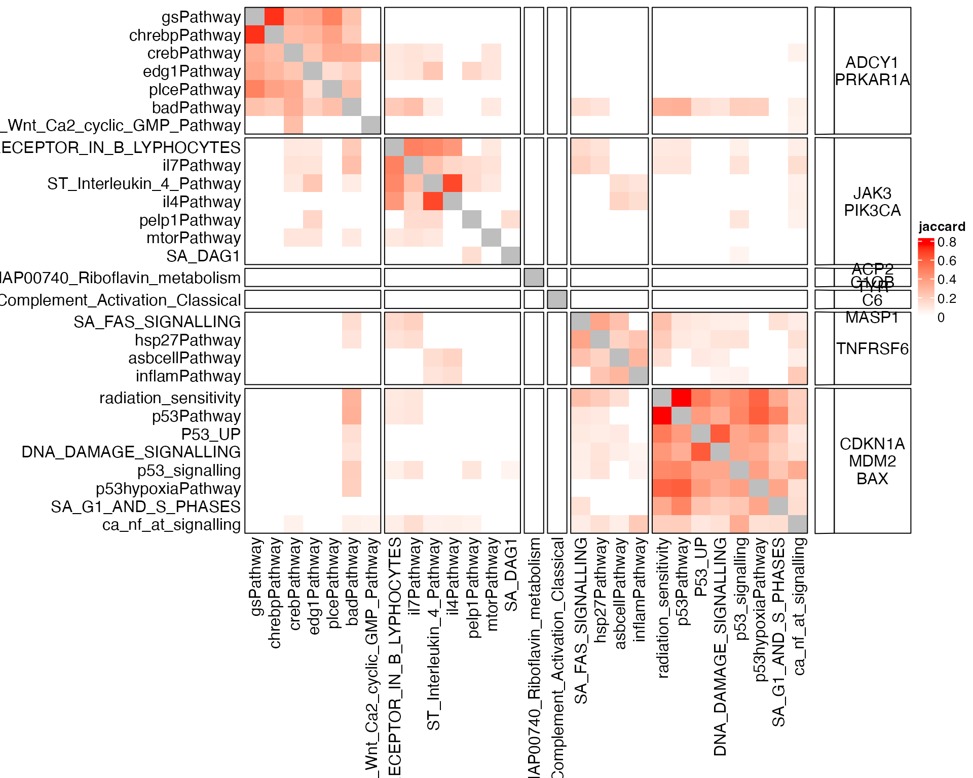
##       1       1       1

We can see “CDKN1A” is in all 8 genesets, “MDM2” is in 7 out of 8 gene sets, and “BAX” is in 6 out of 8 gene sets. So these three genes are driving genes of the eight genesets in this cluster.

For the visualization purpose, can we add such driving genes to the heatmap?

Let’s first adjust the heatmap:

ht = Heatmap(sm, name = "jaccard", col = c("white", "red"), border = "black",
    row_split = cl, column_split = cl, row_names_side = "left",
    show_row_dend = FALSE, show_column_dend = FALSE, row_title = NULL, column_title = NULL)

Driving genes are added as a “link” annotation:

ht + rowAnnotation(gene = anno_link(cl, panel_fun = function(index) {
    tb = table(unlist(gs2[index]))
    tb = sort(tb, decreasing = TRUE)
    pushViewport(viewport())
    grid.rect()
    grid.text(paste(names(tb)[tb/length(index) > 0.5], collapse = "\n"))
    popViewport()
}))

In the GSEAtopics package, there is a genesets_similarity_heatmap() function.

genesets_similarity_heatmap(gs2, weight = w)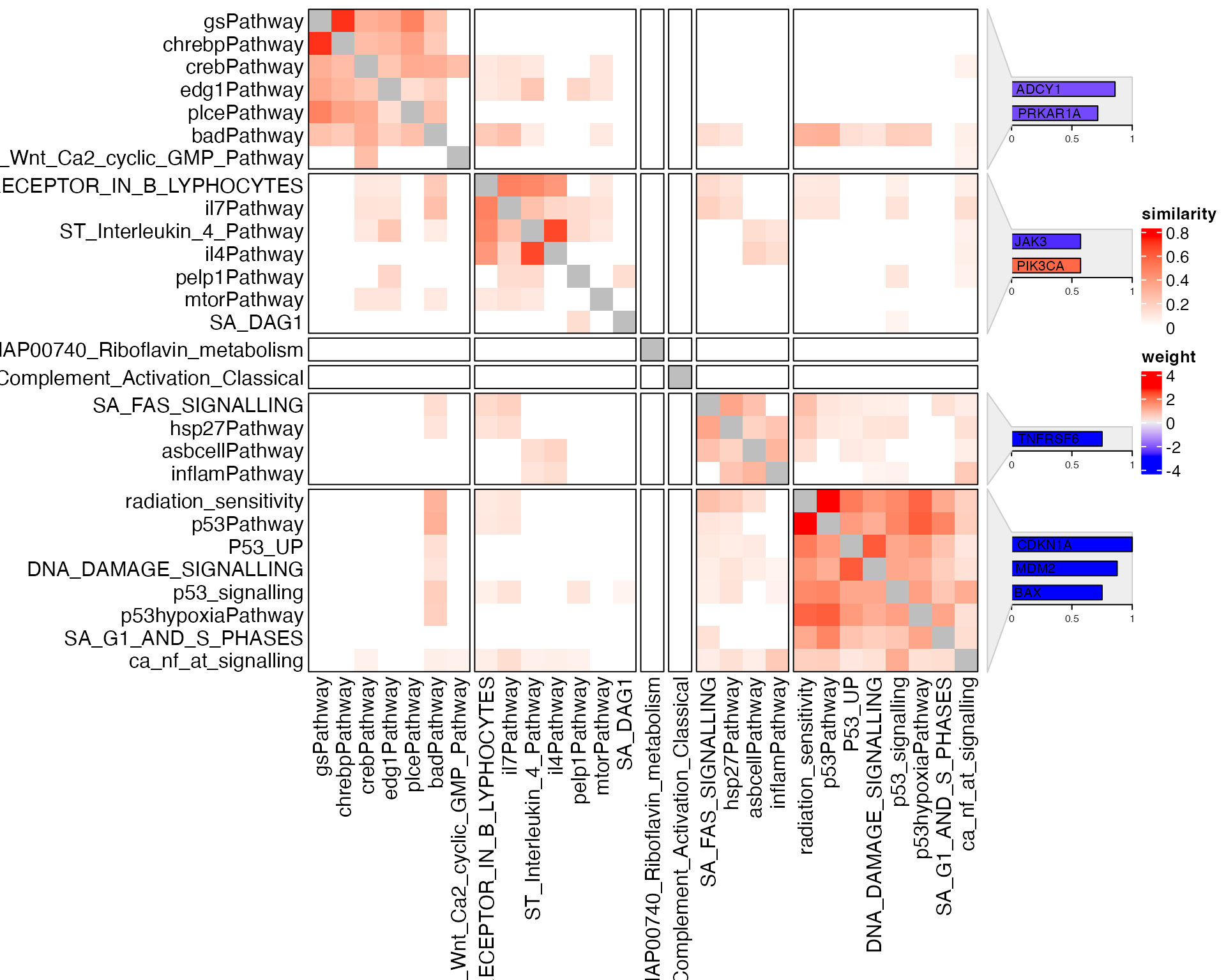

Question: in the previous example, the enrichment is done by ORA which is based on gene counts. The similarity is also based on gene counts. What if the enrichment is done by GSEA? How to adjust the calculation process?

We first apply the GSEA analysis.

s = p53_dataset$s2n
tb_gsea = fgsea_wrapper(s, gs)
head(tb_gsea)

##                       gene_set      p_value    p_adjust log2_p_err         es
## 1                       P53_UP 1.081506e-05 0.002738176  0.5933255 -0.5986774
## 2                 hsp27Pathway 1.113080e-05 0.002738176  0.5933255 -0.7758925
## 3 GPCRs_Class_A_Rhodopsin-like 2.700012e-05 0.003757188  0.5756103 -0.4299558
## 4                   p53Pathway 3.054625e-05 0.003757188  0.5573322 -0.7438596
## 5               UPREG_BY_HOXA9 4.531819e-05 0.004459310  0.5573322  0.5828988
## 6                     HTERT_UP 7.091603e-05 0.005815114  0.5384341  0.3709129
##         nes n_gs leading_edge
## 1 -2.127459   40 CDKN1A, ....
## 2 -2.194198   15 TNFRSF6,....
## 3 -1.853143  111 NTSR2, A....
## 4 -2.132484   16 CDKN1A, ....
## 5  2.213421   29 YES1, TD....
## 6  1.875231  109 AHR, DR1....

The similarity in this category is based on gene counts. Although the enrichment procedure is not gene count-based. In the results, GSEA reports “leading edge genes” which are the genes that contribute most to the enrichment of the gene set. These leading-edge genes can be used for calculating the similarities.

l = tb_gsea$p_adjust < 0.1
gs3 = tb_gsea[l, "leading_edge"]
names(gs3) = tb_gsea$gene_set[l]
genesets_similarity_heatmap(gs3, weight = s, resolution = 1.5)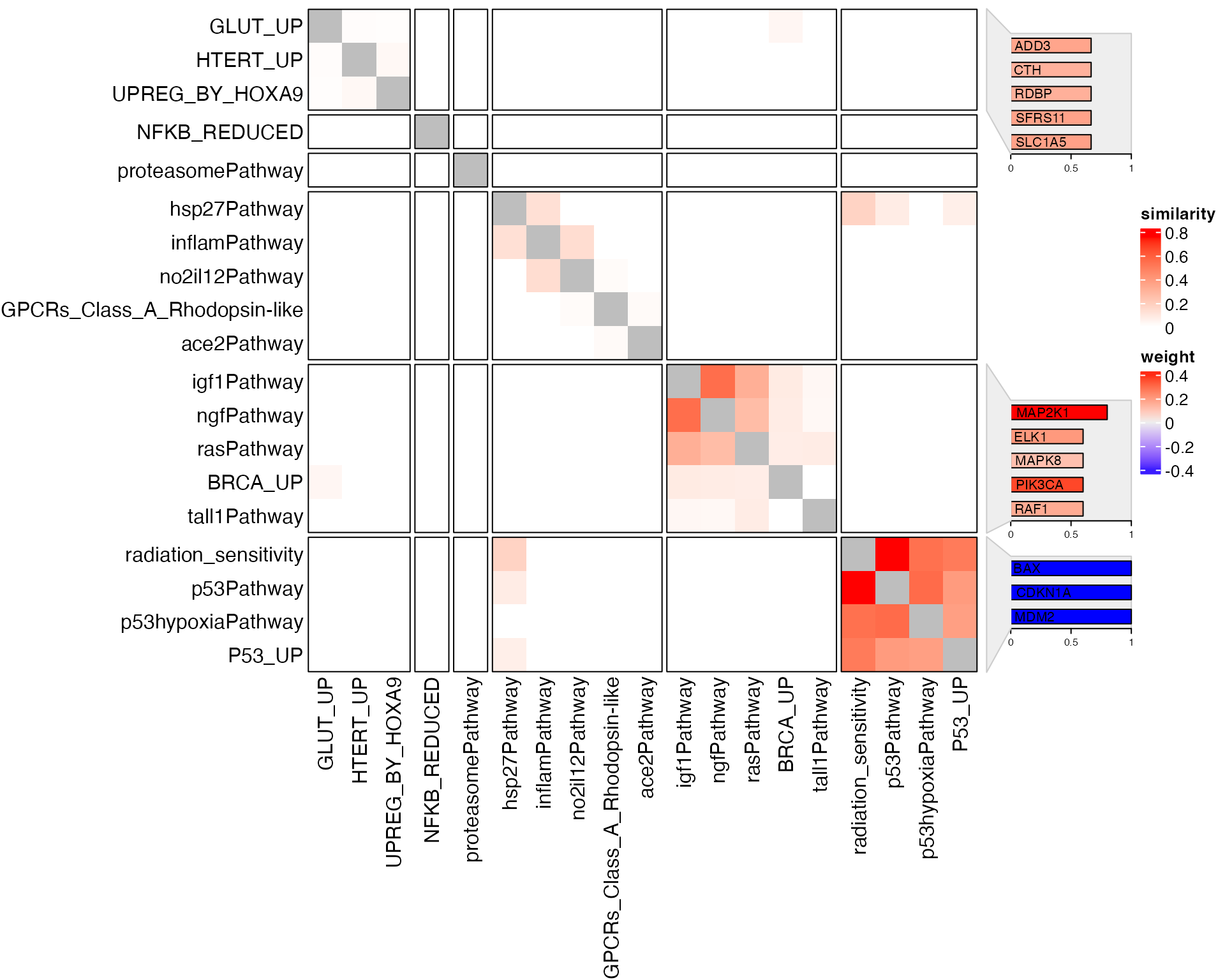

Thoughts: GSVA or the single-sample GSEA converts the original gene-sample matrix to geneset-sample matrix. One the aim of such transformation is to find “co-expressed gene sets”. As such “co-expression” is actually due to common genes in the gene sets, we can also do such driving-gene analysis and associate co-expressed pathways to a group of co-expressed genes.

Semantic similarity

simplifyEnrichment is suggested to work with GO enrichment results.

Let’s generate 500 random GO IDs:

library(simplifyEnrichment)
set.seed(888)
go_id = random_GO(500)
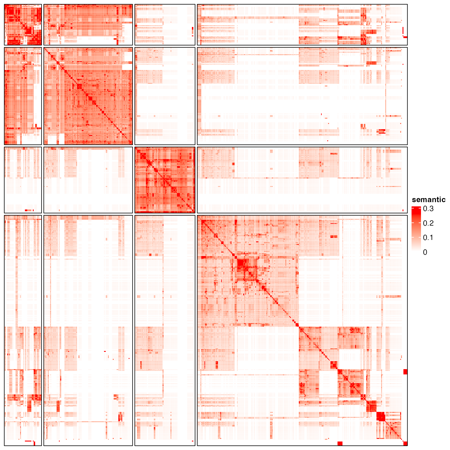
sm = GO_similarity(go_id)

The default semantic similarity method is “Sim_XGraSM_2013”, which is an adjusted Lin-1998 method, where $\mathrm{IC}(\mathrm{MICA})$ is replaced with $\mathrm{avg} \mathrm{IC}(\mathrm{CA})$, i.e. average non-zero IC of all common ancestors.

Heatmap(sm, name = "semantic", col = c("white", "red"))

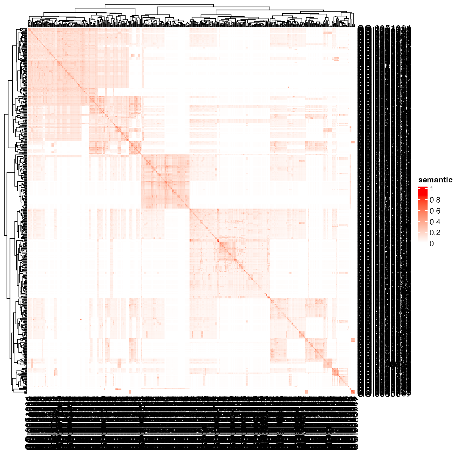
The heatmap shows very clear block patterns on the diagonal. We next try several clustering methods to see whether they can capture such patterns.

We implement a helper function test_clustering() which accepts a cluster label vector and draws the heatmap.

library(circlize)
test_clustering = function(cl) {
    col_fun = colorRamp2(c(0, quantile(sm, 0.99)), c("white", "red"))
    Heatmap(sm, name = "semantic", col = col_fun, 
        border = "black", show_row_names = FALSE, show_column_names = FALSE,
        show_row_dend = FALSE, show_column_dend = FALSE, 
        row_title = NULL, column_title = NULL, row_split = cl, column_split = cl)
}

We try hierarchical cluster, k-means, graph-based method and binary cut.

cl = cutree(hclust(dist(sm)), k = 4)
test_clustering(cl)

cl = kmeans(dist(sm), centers = 4)$cluster
test_clustering(cl)

g = graph_from_adjacency_matrix(sm, weighted = TRUE, mode = "upper", diag = FALSE)
cl = membership(cluster_louvain(g))
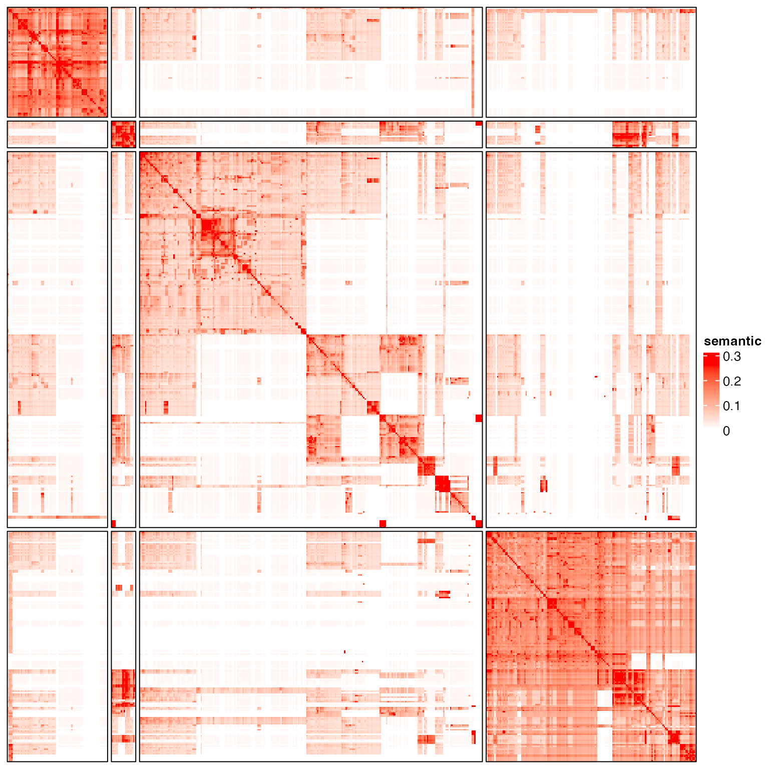
test_clustering(cl)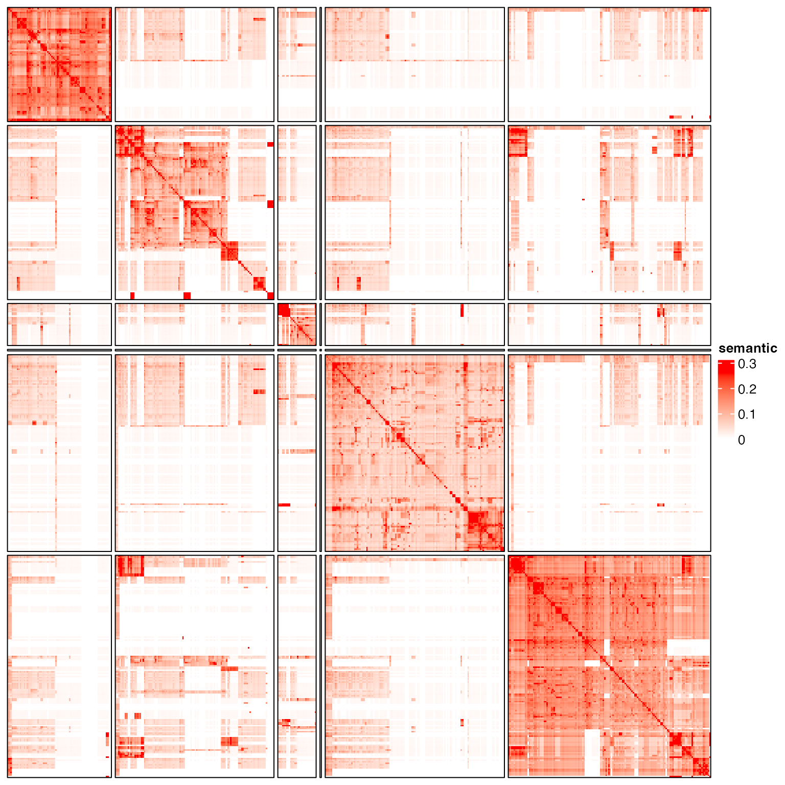

cl = binary_cut(sm)
test_clustering(cl)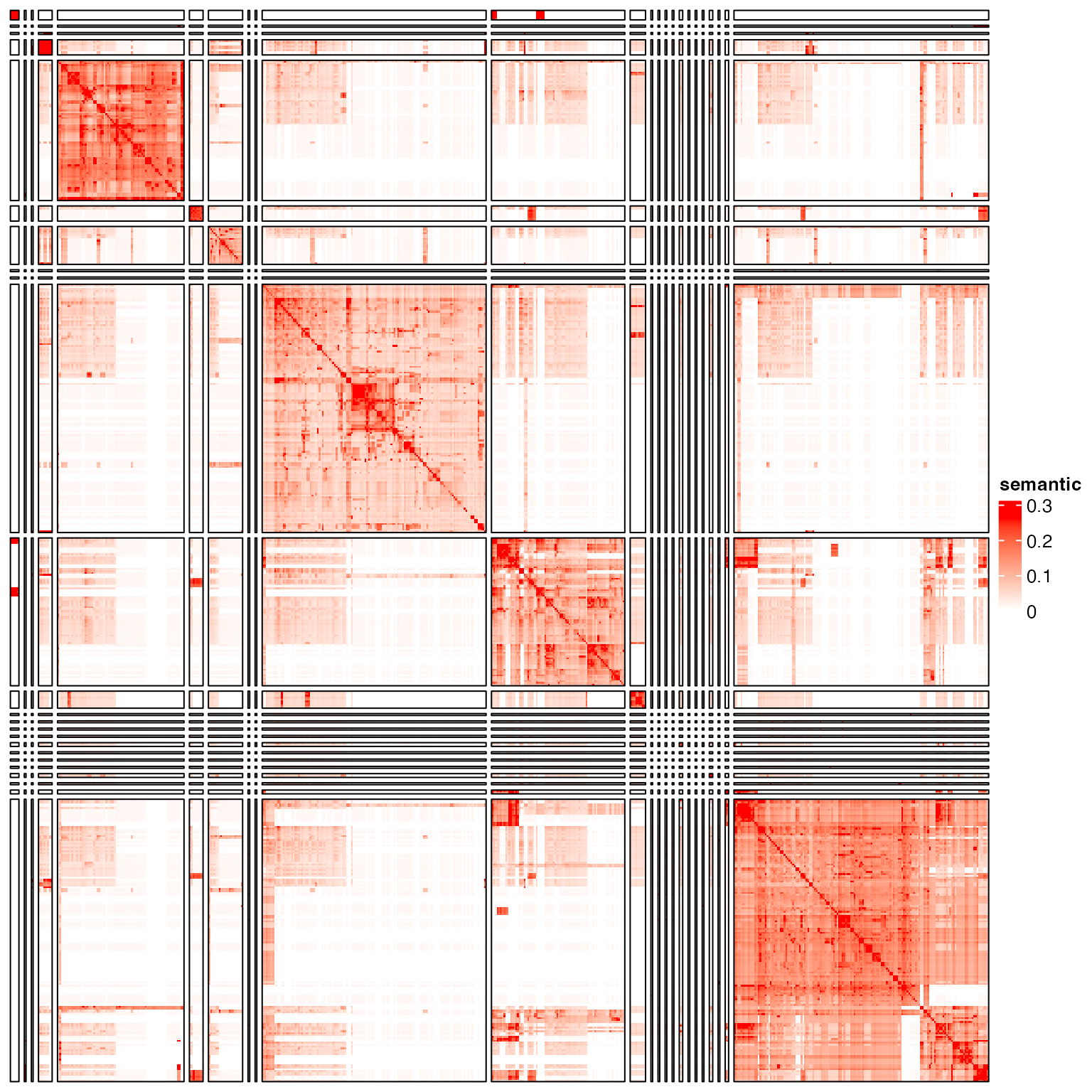

cl = as.character(cl)
tb = table(cl)
cl[cl %in% names(tb[tb < 5])] = "others"
test_clustering(cl)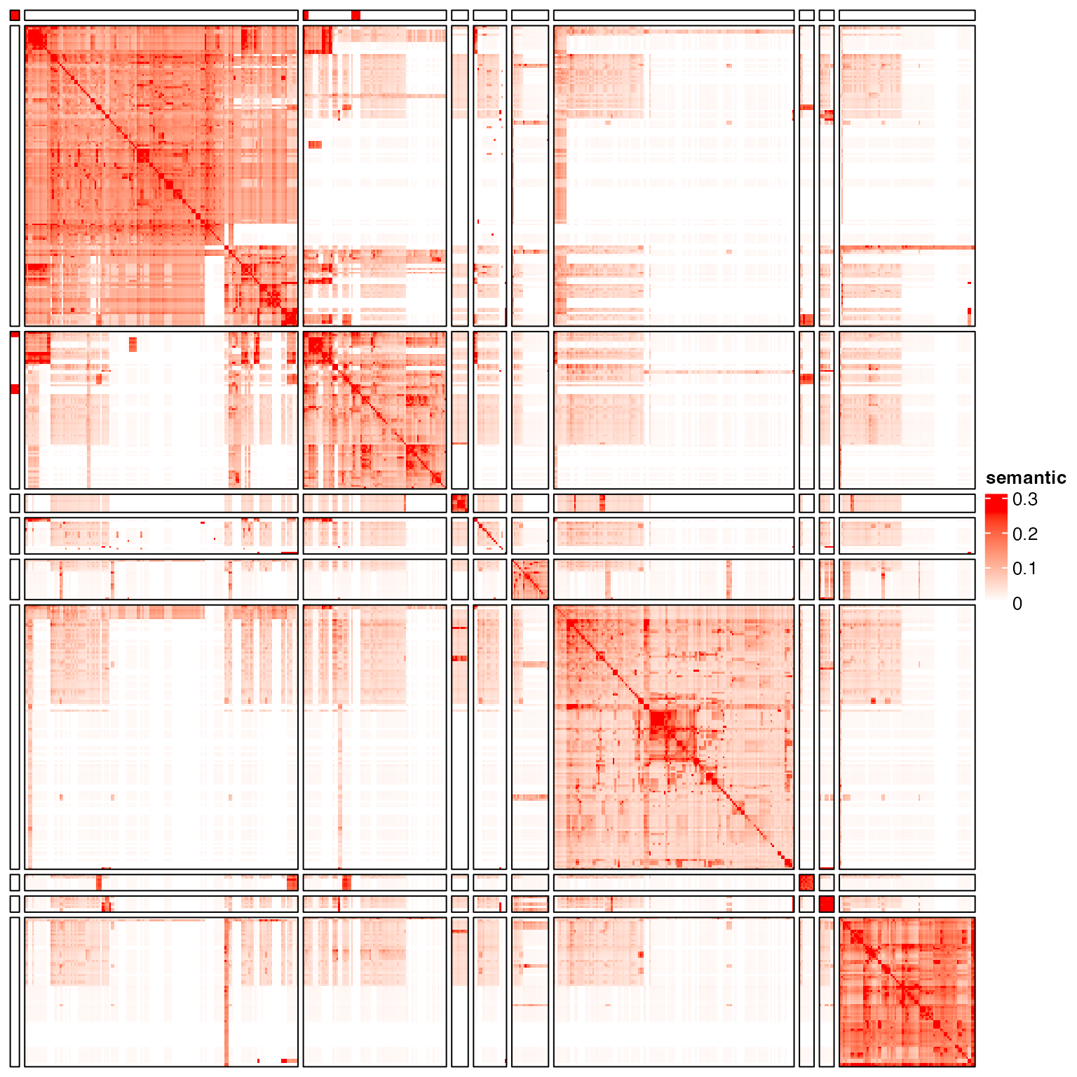

As GO terms in a cluster show high semantic similarities, where they should be concentrated in a certain GO branch. The general biological functions for a GO cluster is summarized by keywords and visualized by word cloud.

simplifyGO(go_id)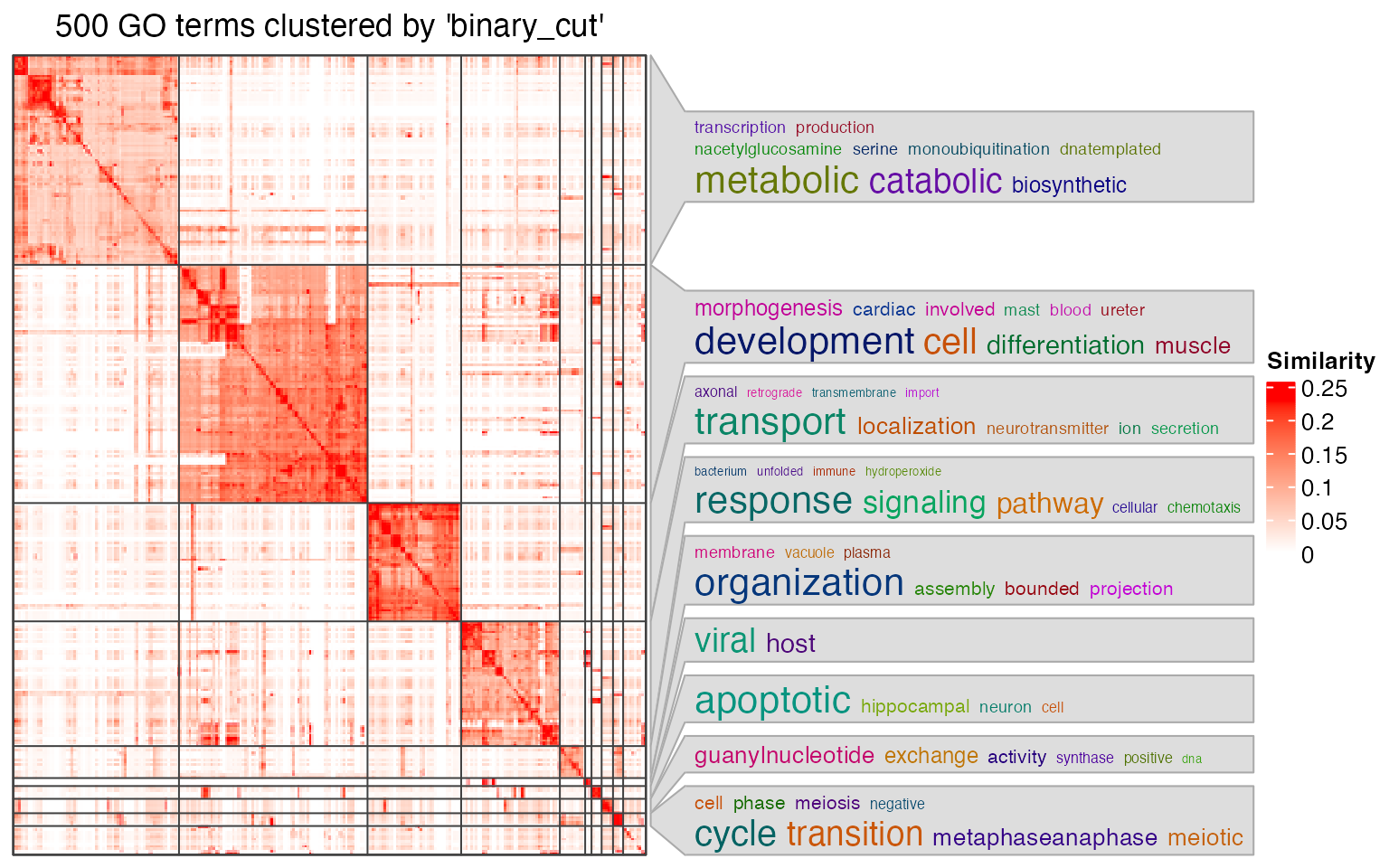

Multiple enrichment results

We follow the standard workflow for unsupervised cluster analysis. We use the Golub ALL dataset and the cola package for analysis.

library(cola)

library(golubEsets)
data(Golub_Merge)
m = exprs(Golub_Merge)

anno = pData(Golub_Merge)

m[m <= 1] = NA
m = log10(m)

m = adjust_matrix(m)

library(preprocessCore)
cn = colnames(m)
rn = rownames(m)
m = normalize.quantiles(m)
colnames(m) = cn
rownames(m) = rn

res = consensus_partition(m, top_value_method = "ATC", partition_method = "skmeans", verbose = FALSE)

We know the best number of subgroups is three. We look for signatures in the three-subgroup classification.

df = get_signatures(res, k = 3)

## * 71/72 samples (in 3 classes) remain after filtering by silhouette (>= 0.5).
## * cache hash: bc6884118a3de686a9e28200827a1400 (seed 888).
## * calculating row difference between subgroups by Ftest.
## * split rows into 4 groups by k-means clustering.
## * 2080 signatures (50.5%) under fdr < 0.05, group_diff > 0.
##   - randomly sample 2000 signatures.
## * making heatmaps for signatures.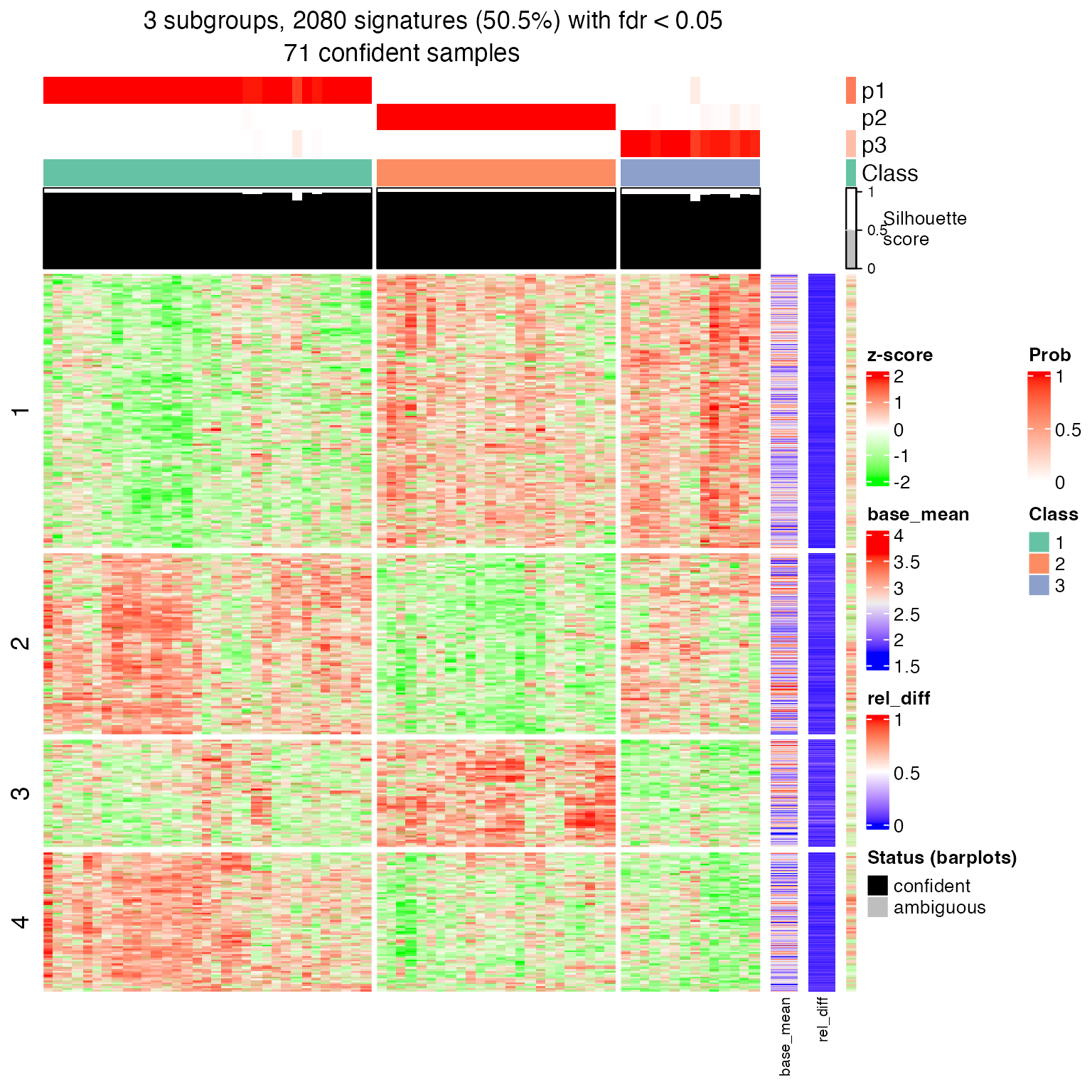

Now we have four groups of signatures genes. The next analysis is to compare enriched GO functions in the four lists of signature genes. The corresponding biological question is do these different signature genes have similar function or they exhibit specific functions?

We first obtain the four list of signature genes.

gl = split(df$which_row, df$km)
gl = lapply(gl, function(ind) rownames(res)[ind])

The ALL data is almost 25 years ago. The gene ID is Affymetric microarray probe ID, Luckily, the corresponding annotation package is also available on Bioconductor which is built upon the standard AnnotationDbi package.

library(hu6800.db)
gl = lapply(gl, function(x) {
    x2 = mapIds(hu6800.db, keys = x, keytype = "PROBEID", column = "ENTREZID")
    unique(x2[!is.na(x2)])
})

We aply ORA GO analysis.

tbl = lapply(gl, ora_go)

tbl is a list of four enrichment result tables. simplifyGOFromMultipleLists() can be used to visualize GO enrichment from multiple results. The columns for GO IDs and p-values are automatically detected.

simplifyGOFromMultipleLists(tbl, padj_cutoff = 0.001)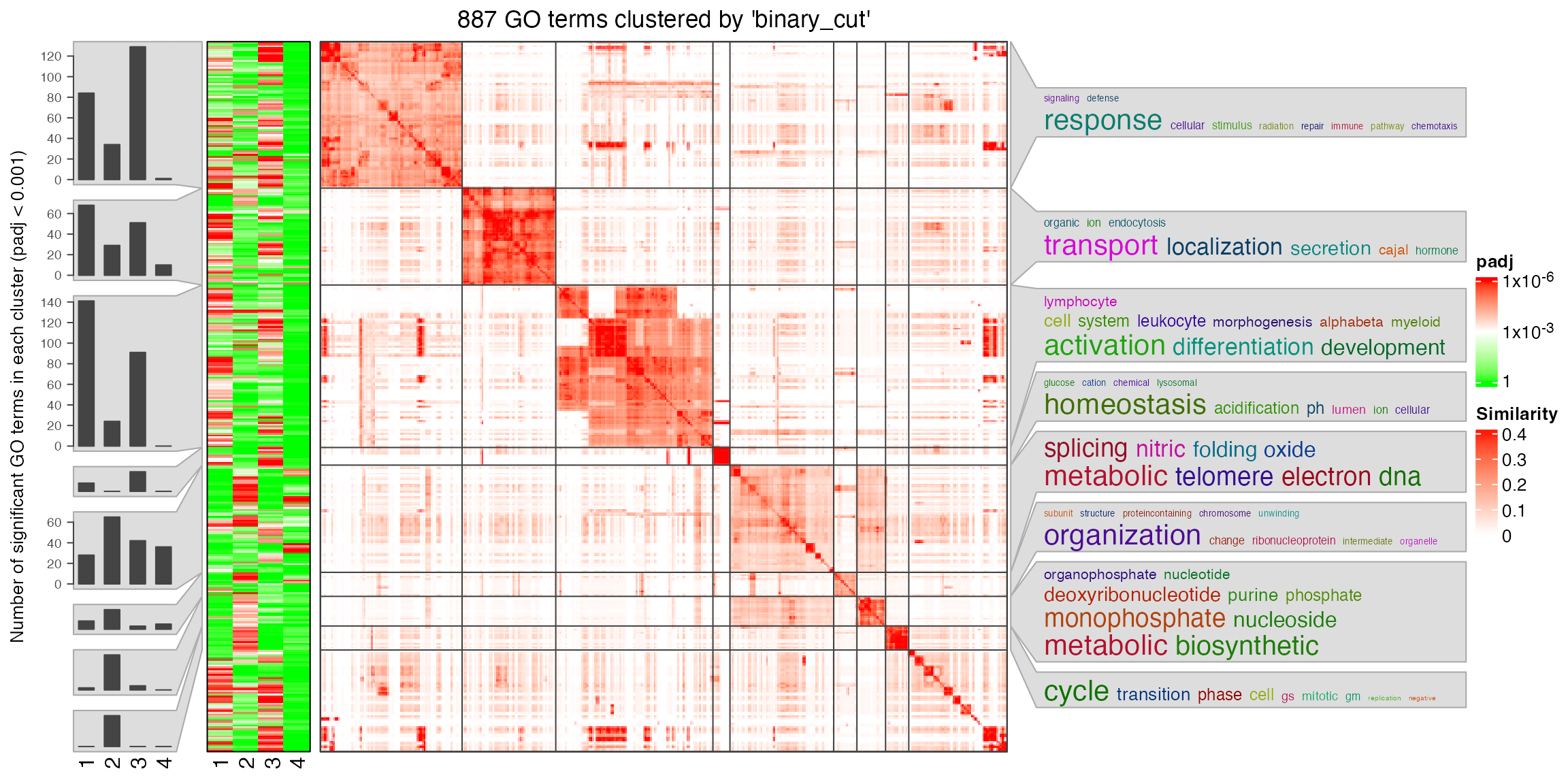

You can see there are around 900 GO terms under the cutoff p_adjust < 0.001. I suggest to set a cutoff for padj_cutoff to let the number of GO terms be in [100, 1000].

Word cloud

In some cases, the similarity heatmap is not necessary to put into the final report.

df = tbl[[1]]
go_id = df$gene_set[df$p_adjust < 0.01]
simplifyGO(go_id)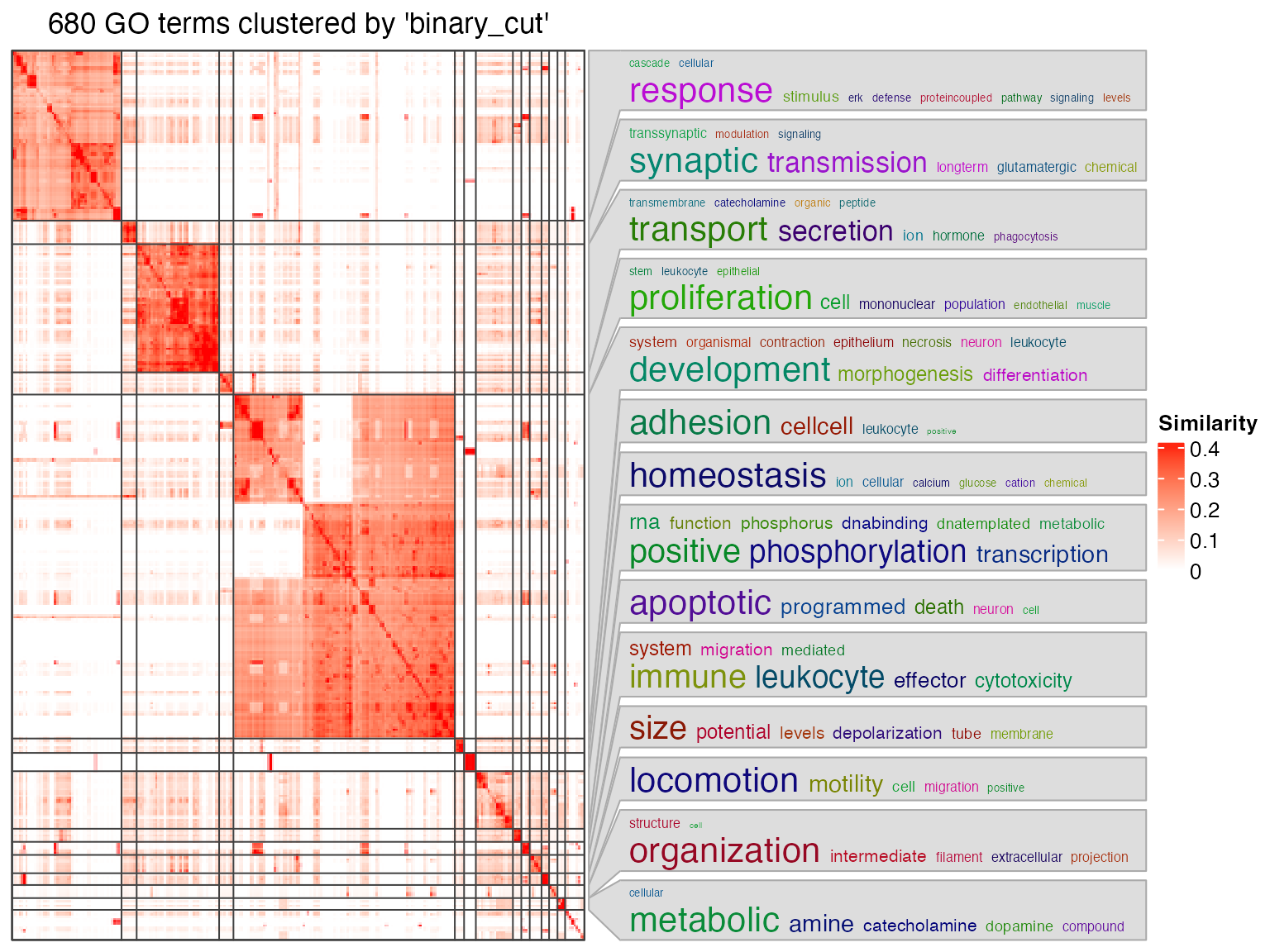

summarizeGO() makes an even simpler plot with word cloud and simple statistical graphics.

When there is only one enrichment results, there are two inputs for summarizeGO():

• A vector of GO IDs
• A numeric vector of corresponding statistics which are mapped to barplots.

l = df$p_adjust < 0.01
summarizeGO(df$gene_set[l], -log10(df$p_adjust)[l], axis_label = "average -log10(p.adjust)")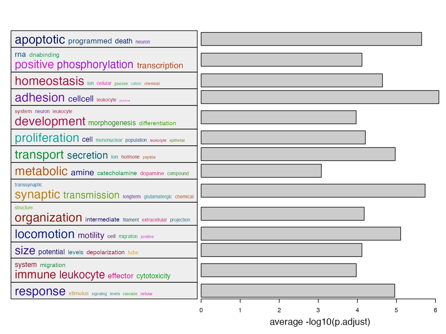

Or visualize average log2 fold enrichment:

l = df$p_adjust < 0.01
summarizeGO(df$gene_set[l], df$log2fe[l], axis_label = "average log2(fold enrichment)")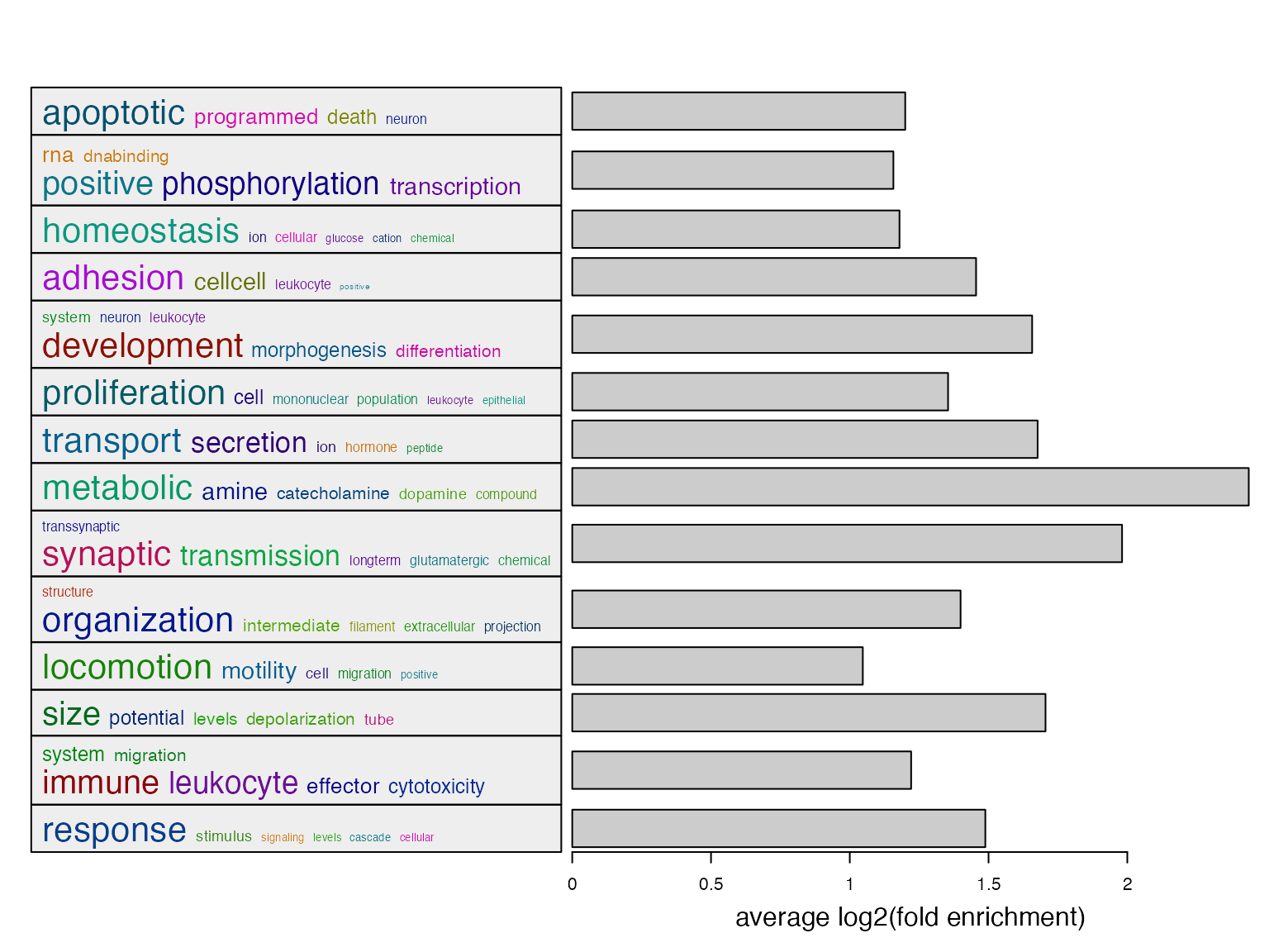

summarizeGO() also supports multiple enrichment results. In this case, value should be is a list of numeric named vectors which contains significant GO terms in each enrichment table.

value = lapply(tbl, function(df) {
    v = -log10(df$p_adjust)
    names(v) = df$gene_set
    v[df$p_adjust < 0.001]
})
str(value)

## List of 4
##  $ 1: Named num [1:420] 26.2 18.9 18.2 15.9 15.7 ...
##   ..- attr(*, "names")= chr [1:420] "GO:1901700" "GO:0007267" "GO:1901701" "GO:0033993" ...
##  $ 2: Named num [1:262] 27.4 20.3 18 16.7 16.5 ...
##   ..- attr(*, "names")= chr [1:262] "GO:0006259" "GO:0006974" "GO:0006281" "GO:1903047" ...
##  $ 3: Named num [1:423] 21.8 20.2 19.9 19.9 19.2 ...
##   ..- attr(*, "names")= chr [1:423] "GO:0044419" "GO:0009607" "GO:0051707" "GO:0043207" ...
##  $ 4: Named num [1:52] 13.9 13.7 13.7 12.9 11.8 ...
##   ..- attr(*, "names")= chr [1:52] "GO:0000375" "GO:0000377" "GO:0000398" "GO:0008380" ...

summarizeGO(value = value, axis_label = "average -log10(p_adjust)", 
    legend_title = "-log10(p_adjust)")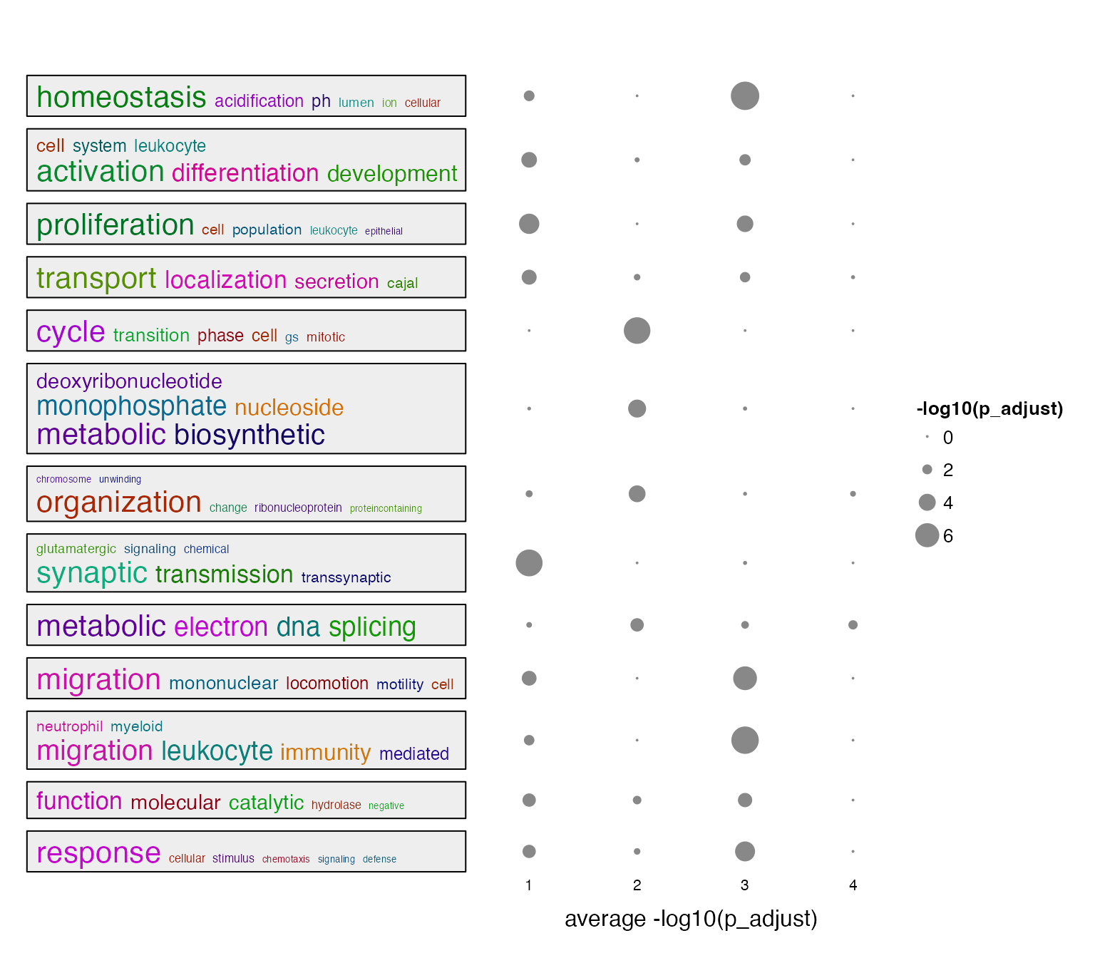

Or use log2 fold enrichment:

value = lapply(tbl, function(df) {
    v = df$log2fe
    names(v) = df$gene_set
    v[df$p_adjust < 0.001]
})
summarizeGO(value = value, axis_label = "average log2_fold_enrichment", 
    legend_title = "log2(fold_enrichment)")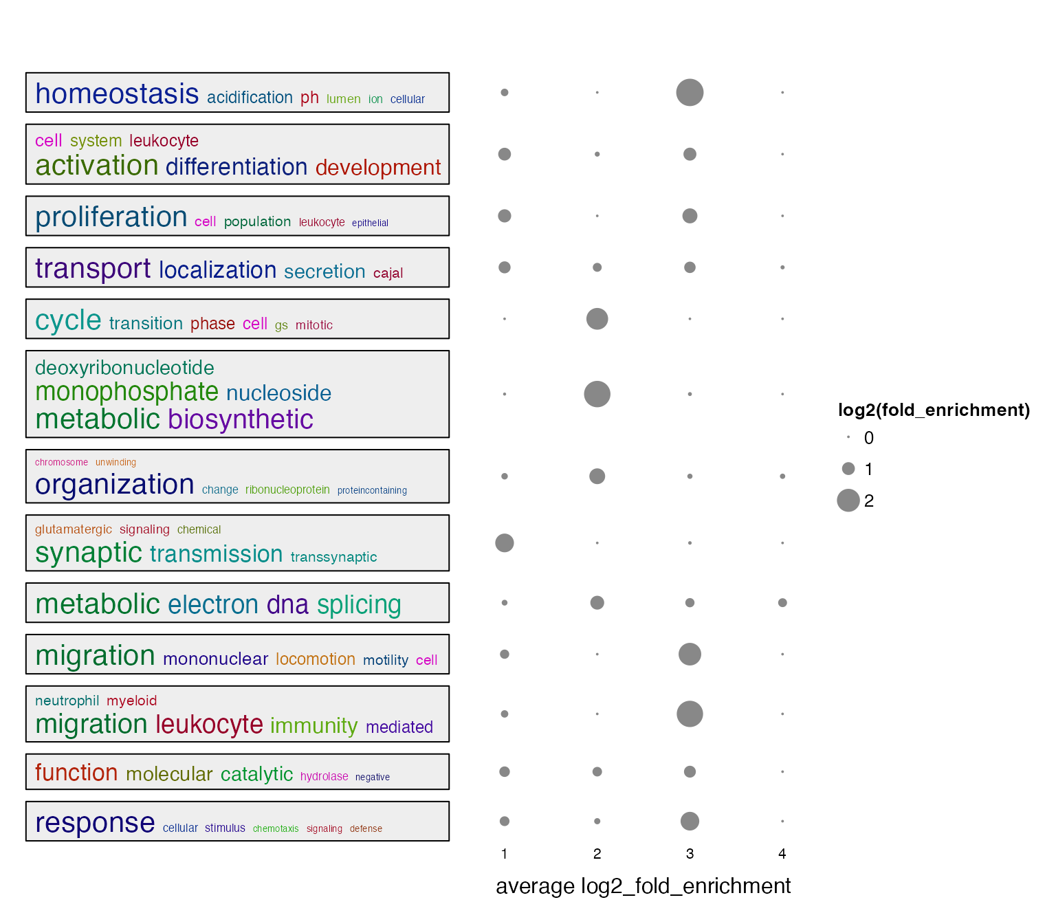

Practice

Practice 1

• Practice
• Solution

Recall in Topic 2-02: Implement ORA from stratch, we compared the ORA results when setting DE cutoffs to 0.05, 0.01 and 0.001. Now perform a simplify enrichment analysis on the three ORA tables and compare them.

de = readRDS(system.file("extdata", "de.rds", package = "GSEAtopics"))
de = de[, c("symbol", "p_value")]
de = de[!is.na(de$p_value) & de$symbol != "", ]

de_genes_1 = de$symbol[de$p_value < 0.05]
de_genes_2 = de$symbol[de$p_value < 0.01]
de_genes_3 = de$symbol[de$p_value < 0.001]

library(org.Hs.eg.db)
map = GSEAtopics::map_to_entrez("SYMBOL", org.Hs.eg.db)

de_genes_1 = unique(map[de_genes_1])
de_genes_1 = de_genes_1[!is.na(de_genes_1)]

de_genes_2 = unique(map[de_genes_2])
de_genes_2 = de_genes_2[!is.na(de_genes_2)]

de_genes_3 = unique(map[de_genes_3])
de_genes_3 = de_genes_3[!is.na(de_genes_3)]

library(org.Hs.eg.db)
gs = load_go_genesets(org.Hs.eg.db, "BP")$gs

tb1 = ora(de_genes_1, gs)
tb2 = ora(de_genes_2, gs)
tb3 = ora(de_genes_3, gs)

lt = list(
    "DE_0.05" = tb1,
    "DE_0.01" = tb2,
    "DE_0.001" = tb3
)

simplifyGOFromMultipleLists(lt, padj_cutoff = 0.05)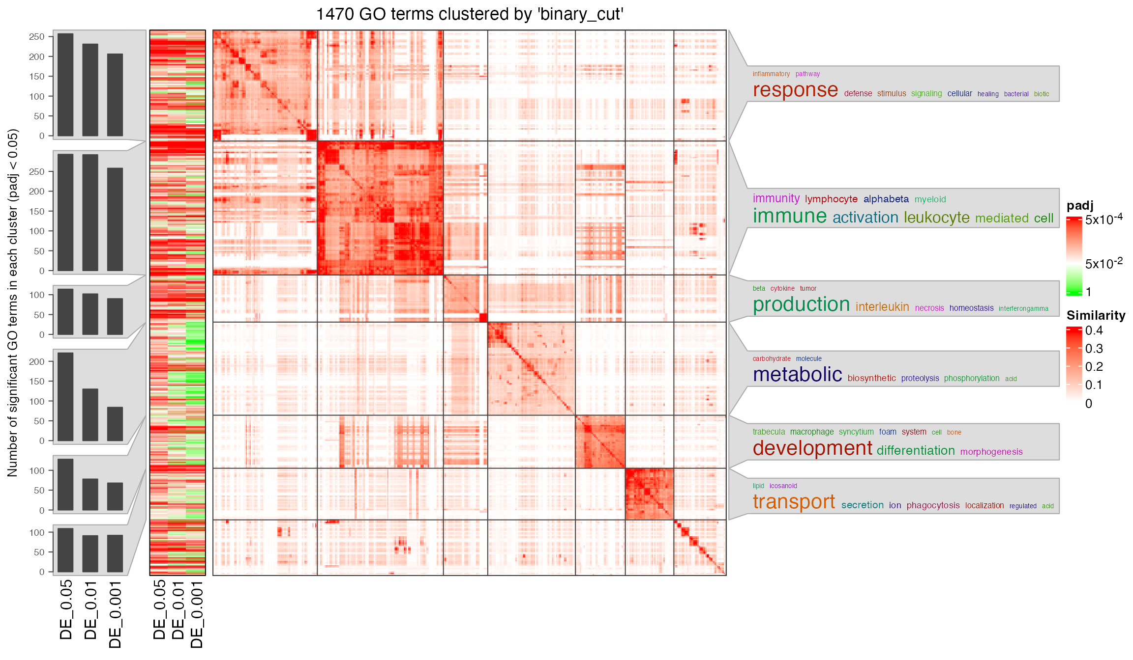

Or taking the average log10 p-values:

value = lapply(lt, function(df) {
    v = -log10(df$p_adjust)
    names(v) = df$gene_set
    v[df$p_adjust < 0.05]
})

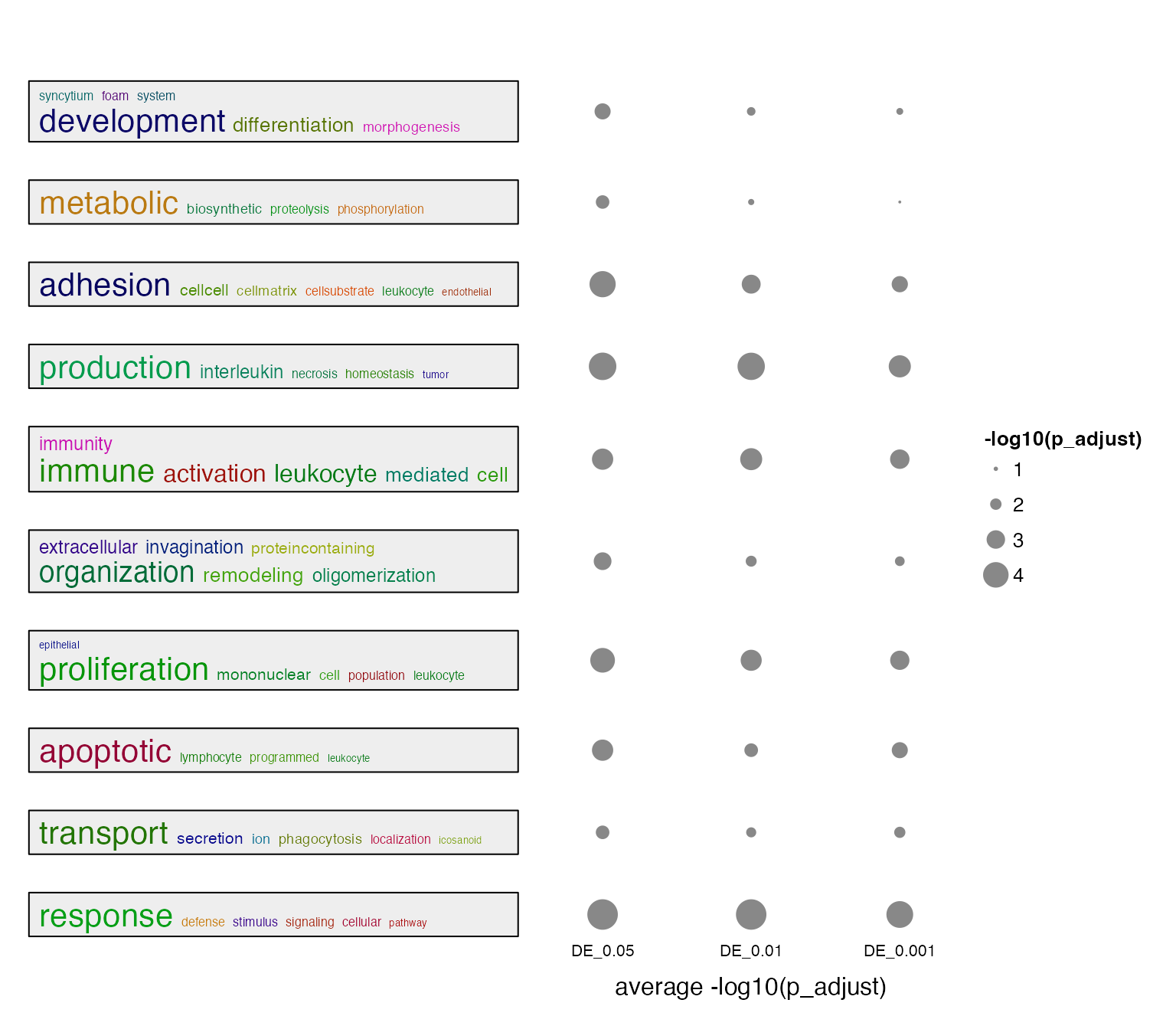
summarizeGO(value = value, axis_label = "average -log10(p_adjust)", 
    legend_title = "-log10(p_adjust)")