Topic 2-02: Implement ORA from scratch

Implementing ORA is very simple. As long as genes and gene sets are already in the correct ID types, the implementation of ORA only needs a few lines of code.

Calculate the statistics

There are three input parameters for ORA:

a vector of (DE) genes: genes
a gene set: gene_set
a vector of background genes: universe

With these three objects, we calculate the following statistics:

The number of total genes:

n_universe = length(universe)

The number of DE genes:

k = length(genes)

The number of genes in each gene set, i.e., the size of each gene set:

m = length(gene_set)

And, the number of DE genes in gene sets:

x = length(intersect(gene_set, genes))

We put these variables into the 2x2 contigency table:

	in the set	not in the set	total
DE	`x`	-	`k`
not DE	-	-	-
total	`m`	-	`n_universe`

Then we can calculate the p-value from the hypergeometric distribution as:

phyper(x - 1, m, n_universe - m, k, lower.tail = FALSE)

which is the same as:

phyper(x - 1, k, n_universe - k, m, lower.tail = FALSE)

Note, phyper() calculates $P(X > x)$ , thus we write phyper(x - 1, ...) which corresponds to $P(X > x - 1) = P(X \ge x)$ .

Wrap into a function

We use a list of random DE genes and GO BP gene sets for testing.

library(org.Hs.eg.db)
library(GSEAtopics)
lt = load_go_genesets(org.Hs.eg.db, "BP")
gs_go = lt$gs

genes = random_genes(org.Hs.eg.db, 1000)
universe = protein_coding_genes(org.Hs.eg.db)

A quick and dirty way by first implementing a function working on single gene set, then applying it to a list of gene sets.

ora_single = function(genes, gene_set, universe) {
    n_universe = length(universe)
    k = length(genes)
    
    x = length(intersect(gene_set, genes))
    m = length(gene_set)
    n = n_universe - m
    
    p = phyper(x - 1, m, n, k, lower.tail = FALSE)

    p
}

ora =  function(genes, gene_sets, universe) {
    ns = length(gene_sets)
    p = numeric(ns)
    for(i in seq_along(gene_sets)) {
        p[i] = ora_single(genes, gene_sets[[i]], universe)
    }
    p
}
ora(genes, gs_go, universe) |> head()

## [1] 0.7755099 0.1458202 1.0000000 0.6989436 1.0000000 1.0000000

Or we can do it in a vectorized way. We also wrap the results as a data frame not only reporting p-values.

ora = function(genes, gene_sets, universe) {
    n_universe = length(universe)
    k = length(genes)
    
    x = sapply(gene_sets, function(x) length(intersect(x, genes)))
    m = sapply(gene_sets, length)
    n = n_universe - m
    
    p = phyper(x - 1, m, n, k, lower.tail = FALSE)

    data.frame(
        gene_set = names(gene_sets),
        n_hits = x,
        n_genes = k,
        n_gs = m,
        n_total = n_universe,
        p_value = p
    )
}
ora(genes, gs_go, universe) |> head()

##              gene_set n_hits n_genes n_gs n_total   p_value
## GO:0000002 GO:0000002      1    1000   30   20600 0.7755099
## GO:0000012 GO:0000012      2    1000   14   20600 0.1458202
## GO:0000017 GO:0000017      0    1000    2   20600 1.0000000
## GO:0000018 GO:0000018      6    1000  143   20600 0.6989436
## GO:0000019 GO:0000019      0    1000    7   20600 1.0000000
## GO:0000022 GO:0000022      0    1000   12   20600 1.0000000

We can further improve the function by:

setting the default of universe to the total genes in gene_sets,
intersecting genes and gene_sets to universe. Note this step also removes duplicated genes,
adding log2 fold enrichment and adjusted p-values to the result data frame,
ordering the result data frame by the significance.

ora = function(genes, gene_sets, universe = NULL) {

    if(is.null(universe)) {
        universe = unique(unlist(gene_sets))
    } else {
        universe = unique(universe)
    }

    genes = intersect(genes, universe)
    gene_sets = lapply(gene_sets, function(x) intersect(x, universe))

    n_universe = length(universe)
    k = length(genes)
    
    x = sapply(gene_sets, function(x) length(intersect(x, genes)))
    m = sapply(gene_sets, length)
    n = n_universe - m
    
    p = phyper(x - 1, m, n, k, lower.tail = FALSE)

    df = data.frame(
        gene_set = names(gene_sets),
        n_hits = x,
        n_genes = k,
        n_gs = m,
        n_universe = n_universe,
        log2fe = log2(x*n_universe/k/m),
        p_value = p
    )

    df$p_adjust = p.adjust(df$p_value, "BH")
    df[order(df$p_adjust, df$p_value), ,drop = FALSE]
}
ora(genes, gs_go) |> head()

##              gene_set n_hits n_genes n_gs n_universe   log2fe     p_value
## GO:0000350 GO:0000350      2     854    2      18986 4.474556 0.002020984
## GO:0018993 GO:0018993      2     854    2      18986 4.474556 0.002020984
## GO:0036145 GO:0036145      2     854    2      18986 4.474556 0.002020984
## GO:0032011 GO:0032011      5     854   21      18986 2.404167 0.002027995
## GO:0032012 GO:0032012      5     854   21      18986 2.404167 0.002027995
## GO:0010572 GO:0010572      4     854   13      18986 2.774116 0.002097904
##            p_adjust
## GO:0000350        1
## GO:0018993        1
## GO:0036145        1
## GO:0032011        1
## GO:0032012        1
## GO:0010572        1

Further optimization

Why do we need to further optimize ORA? The hypergeometric method is not only used in ORA, but is more like an universal method. In many cases, the tests are applied for a huge number of times (> thousands). Also the methods for optimization can be applied to a large number of other scenarios.

We first rename ora() to ora_old() later for comparison.

ora_old = ora

ora() is already very fast. However, in the previous implementation, there is still a part which is relatively slow in the function. Let’t first do a code profiling.

Rprof()
df = ora(genes, gs_go)
Rprof(NULL)
summaryRprof()

## $by.self
##                      self.time self.pct total.time total.pct
## "base::intersect"         2.22    93.28       2.28     95.80
## "unlist"                  0.08     3.36       0.08      3.36
## "duplicated.default"      0.06     2.52       0.06      2.52
## "unique.default"          0.02     0.84       0.02      0.84
## 
## $by.total
##                             total.time total.pct self.time self.pct
## "<Anonymous>"                     2.38    100.00      0.00     0.00
## "base::do.call"                   2.38    100.00      0.00     0.00
## "base::saveRDS"                   2.38    100.00      0.00     0.00
## "base::tryCatch"                  2.38    100.00      0.00     0.00
## "base::withCallingHandlers"       2.38    100.00      0.00     0.00
## "block_exec"                      2.38    100.00      0.00     0.00
## "call_block"                      2.38    100.00      0.00     0.00
## "doTryCatch"                      2.38    100.00      0.00     0.00
## "doWithOneRestart"                2.38    100.00      0.00     0.00
## "eng_r"                           2.38    100.00      0.00     0.00
## "eval"                            2.38    100.00      0.00     0.00
## "evaluate"                        2.38    100.00      0.00     0.00
## "evaluate::evaluate"              2.38    100.00      0.00     0.00
## "in_dir"                          2.38    100.00      0.00     0.00
## "in_input_dir"                    2.38    100.00      0.00     0.00
## "knitr::knit"                     2.38    100.00      0.00     0.00
## "ora"                             2.38    100.00      0.00     0.00
## "process_file"                    2.38    100.00      0.00     0.00
## "process_group"                   2.38    100.00      0.00     0.00
## "rmarkdown::render"               2.38    100.00      0.00     0.00
## "tryCatchList"                    2.38    100.00      0.00     0.00
## "tryCatchOne"                     2.38    100.00      0.00     0.00
## "withCallingHandlers"             2.38    100.00      0.00     0.00
## "withOneRestart"                  2.38    100.00      0.00     0.00
## "withRestartList"                 2.38    100.00      0.00     0.00
## "withRestarts"                    2.38    100.00      0.00     0.00
## "withVisible"                     2.38    100.00      0.00     0.00
## "with_handlers"                   2.38    100.00      0.00     0.00
## "xfun:::handle_error"             2.38    100.00      0.00     0.00
## "base::intersect"                 2.28     95.80      2.22    93.28
## "FUN"                             2.28     95.80      0.00     0.00
## "intersect"                       2.28     95.80      0.00     0.00
## "lapply"                          2.28     95.80      0.00     0.00
## "sapply"                          0.18      7.56      0.00     0.00
## "unique"                          0.10      4.20      0.00     0.00
## "unlist"                          0.08      3.36      0.08     3.36
## "duplicated.default"              0.06      2.52      0.06     2.52
## "duplicated"                      0.06      2.52      0.00     0.00
## "unique.default"                  0.02      0.84      0.02     0.84
## 
## $sample.interval
## [1] 0.02
## 
## $sampling.time
## [1] 2.38

We can see the intersect() function consumes more than 90% of the total runtime. intersect() internally uses the match() function, and there is a faster implementation in the fastmatch package. We also optimize the use of the unlist() function by adding one additional argument use.names = FALSE since we do not care about the names of the unlisted vector.

library(fastmatch)
ora = function(genes, gene_sets, universe = NULL) {

    if(is.null(universe)) {
        universe = unique(unlist(gene_sets, use.names = FALSE))
    } else {
        universe = unique(universe)
    }
    
    genes = intersect(genes, universe)
    gene_sets = lapply(gene_sets, function(x) x[x %fin% universe])

    n_universe = length(universe)
    k = length(genes)
    
    x = sapply(gene_sets, function(x) sum(x %fin% genes))
    m = sapply(gene_sets, length)
    n = n_universe - m
    
    p = phyper(x - 1, m, n, k, lower.tail = FALSE)

    df = data.frame(
        gene_set = names(gene_sets),
        n_hits = x,
        n_genes = k,
        n_gs = m,
        n_total = n_universe,
        log2fe = log2(x*n_universe/k/m),
        p_value = p
    )

    df$p_adjust = p.adjust(df$p_value, "BH")
    df[order(df$p_adjust, df$p_value), ,drop = FALSE]
}

Now let’s benchmark ora_old() and the new ora():

library(microbenchmark)
microbenchmark(
    ora_old = ora_old(genes, gs_go),
    ora = ora(genes, gs_go),
    times = 10
)

## Unit: milliseconds
##     expr        min         lq       mean     median        uq        max neval
##  ora_old 2449.29187 2469.86628 2536.55297 2547.21071 2580.7377 2617.07924    10
##      ora   54.59093   55.30953   61.09419   55.71064   70.7915   80.50662    10

ora() is more than 40x faster than ora_old()! We have a very faster implementation of ORA than majority of others from R/Bioconductor.

There is still 5% ~ 10% space for further optimization. Note in the previous ora(), x %fin% universe actually matches between two character vectors (internally by hash tables). If we can change it to match between two integer vectors, it might further improve the code.

In the next improved implementation, we still use fmatch() to perform fast matching. We change genes in objects genes and gene_sets all to the corresponding integer indicies in universe. This is done by fmatch().

ora_int = function(genes, gene_sets, universe = NULL) {

    if(is.null(universe)) {
        universe = unique(unlist(gene_sets, use.names = FALSE))
    } else {
        universe = unique(universe)
    }

    # convert genes to integer indicies
    genes = fmatch(genes, universe); genes = genes[!is.na(genes)]
    gene_sets = lapply(gene_sets, function(x) {
        v = fmatch(x, universe)
        v[!is.na(v)]
    })

    n_universe = length(universe)
    k = length(genes)
    
    x = sapply(gene_sets, function(x) sum(x %fin% genes)) # now %fin% is applied on integer vectors
    m = sapply(gene_sets, length)
    n = n_universe - m
    
    p = phyper(x - 1, m, n, k, lower.tail = FALSE)

    df = data.frame(
        gene_set = names(gene_sets),
        n_hits = x,
        n_genes = k,
        n_gs = m,
        n_total = n_universe,
        log2fe = log2(x*n_universe/k/m),
        p_value = p
    )

    df$p_adjust = p.adjust(df$p_value, "BH")
    rownames(df) = df$gene_set
    df[order(df$p_adjust, df$p_value), ,drop = FALSE]
}

microbenchmark(
    ora  = ora(genes, gs_go),
    ora_int = ora_int(genes, gs_go),
    times = 10
)

## Unit: milliseconds
##     expr      min       lq     mean   median       uq      max neval
##      ora 54.65694 56.03138 61.26719 57.15263 68.20006 69.71923    10
##  ora_int 51.94315 53.20435 58.65443 57.23924 63.88866 67.43676    10

And this is how GSEAtopics::ora() is optimized.

Practice

Practice 1

The file de.rds contains results from a differential expression (DE) analysis.

de = readRDS(system.file("extdata", "de.rds", package = "GSEAtopics"))
de = de[, c("symbol", "p_value")]
de = de[!is.na(de$p_value) & de$symbol != "", ]
head(de)

##     symbol      p_value
## 1   TSPAN6 0.0081373337
## 2     TNMD 0.0085126916
## 3     DPM1 0.9874656931
## 4    SCYL3 0.2401551938
## 5 C1orf112 0.8884603214
## 6      FGR 0.0006134791

Take the symbol and p_value columns, set cutoff of p_value to 0.05, 0.01 and 0.001 respectively to filter the significant DE genes (of course, in realworld applications, you need to correct p-values), apply ora() to the three DE gene lists using the GO BP gene sets and compare the three ORA results.

You can use symbols for genes, then you need to generate GO BP genes sets also in gene symbols.
You can use EntreZ IDs for genes, then you need to convert genes in de to EntreZ IDs.

The three DE gene lists:

de_genes_1 = de$symbol[de$p_value < 0.05]
de_genes_2 = de$symbol[de$p_value < 0.01]
de_genes_3 = de$symbol[de$p_value < 0.001]

Since genes are in symbols, we first obtain a global mapping from symbols to EntreZ IDs:

map = map_to_entrez("SYMBOL", org.Hs.eg.db)

de_genes_1 = unique(map[de_genes_1])
de_genes_1 = de_genes_1[!is.na(de_genes_1)]

de_genes_2 = unique(map[de_genes_2])
de_genes_2 = de_genes_2[!is.na(de_genes_2)]

de_genes_3 = unique(map[de_genes_3])
de_genes_3 = de_genes_3[!is.na(de_genes_3)]

Number of DE genes in the three settings:

length(de_genes_1)

## [1] 2568

length(de_genes_2)

## [1] 1415

length(de_genes_3)

## [1] 685

Get the GO BP gene sets.

library(GSEAtopics)
gs = load_go_genesets(org.Hs.eg.db, "BP")$gs
gs[1]

## $`GO:0000002`
##  [1] "142"    "291"    "1763"   "1890"   "2021"   "3980"   "4205"   "4358"  
##  [9] "4976"   "5428"   "6240"   "6742"   "7156"   "7157"   "9093"   "9361"  
## [17] "10000"  "11232"  "50484"  "55186"  "56652"  "64863"  "80119"  "83667" 
## [25] "84275"  "84461"  "92667"  "131474" "201973" "219736"

We perform ORA for the three DE gene lists.

tb1 = ora(de_genes_1, gs)
tb2 = ora(de_genes_2, gs)
tb3 = ora(de_genes_3, gs)

Compare number of significant GO terms:

sum(tb1$p_adjust < 0.05)

## [1] 1197

sum(tb2$p_adjust < 0.05)

## [1] 977

sum(tb3$p_adjust < 0.05)

## [1] 891

The numbers of significant GO terms are very comparible.

Make a Venn (Euler) diagram of the significant GO terms:

library(eulerr)
plot(euler(list("DE_cutoff_0.05"  = tb1$gene_set[tb1$p_adjust < 0.05],
                "DE_cutoff_0.01"  = tb2$gene_set[tb2$p_adjust < 0.05],
                "DE_cutoff_0.001" = tb3$gene_set[tb3$p_adjust < 0.05])), 
     quantities = TRUE)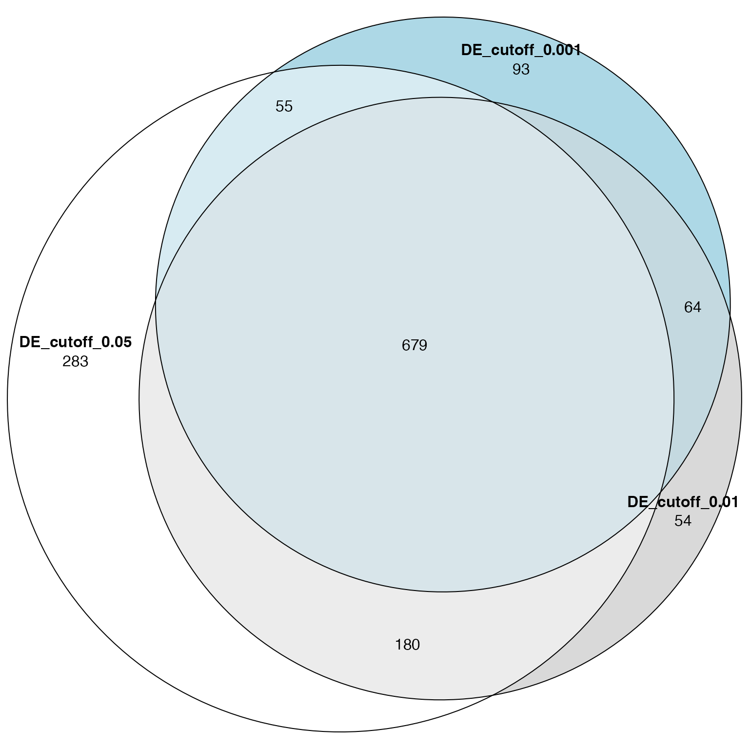

And the Venn diagram for DE genes:

plot(euler(list("DE_cutoff_0.05"  = de_genes_1,
                "DE_cutoff_0.01"  = de_genes_2,
                "DE_cutoff_0.001" = de_genes_3)), 
     quantities = TRUE)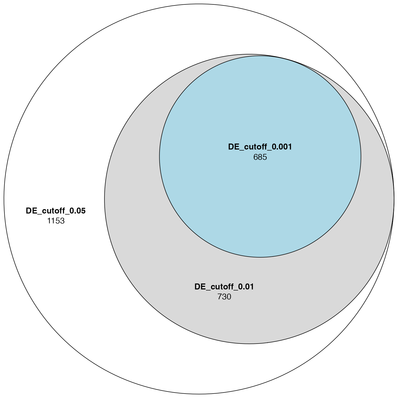

We could roughly conclude that ORA is more robust than DE analysis.

Practice 2

The ora() function can be used as the core part of a full-functional function for ORA analysis. Please implement a ora_go() for GO analysis or a ora_kegg() for KEGG pathway analysis. Following are two templates of the two functions.

ora_go = function(genes, org_db, ontology) {
    # generate go gene sets
    # apply ora()
}

org_db and ontology are used to retrieve GO gene sets for a specific namespace.

ora_kegg = function(genes, organism) {
    # generate kegg gene sets
    # apply ora()
}

organism is the organism code.

To make it simple, we assume genes is always in EntreZ ID type.

ora_go = function(genes, org_db = org.Hs.eg.db, ontology = "BP") {
    tb = AnnotationDbi::select(org_db, keys = ontology, keytype = "ONTOLOGYALL", 
        columns = c("ENTREZID", "GOALL"))
    gs = split(tb$ENTREZID, tb$GOALL)
    gs = lapply(gs, function(x) {
        as.character(unique(x))
    })

    ora(genes, gs)
}

ora_kegg = function(genes, organism = "hsa") {
    pathway_genes = read.table(url(paste0("https://rest.kegg.jp/link/pathway/", organism)), 
        sep = "\t", quote = "")
    pathway_genes[, 1] = gsub("^\\w+:", "", pathway_genes[, 1])
    pathway_genes[, 2] = gsub("^\\w+:", "", pathway_genes[, 2])
    pathway_genes = split(pathway_genes[, 1], pathway_genes[, 2])
        
    ora(genes, pathway_genes)
}

Let’s test these two ora_*() functions.

genes = random_genes(org.Hs.eg.db, 1000)
head(ora_go(genes))

##              gene_set n_hits n_genes n_gs n_total    log2fe      p_value
## GO:0032956 GO:0032956     31     831  352   18986 1.0087084 0.0001838150
## GO:0030036 GO:0030036     54     831  744   18986 0.7296724 0.0001913197
## GO:0051148 GO:0051148     11     831   72   18986 1.8034503 0.0002778395
## GO:0045608 GO:0045608      3     831    4   18986 4.0989062 0.0003233084
## GO:0045632 GO:0045632      3     831    4   18986 4.0989062 0.0003233084
## GO:2000981 GO:2000981      3     831    4   18986 4.0989062 0.0003233084
##             p_adjust
## GO:0032956 0.7007671
## GO:0030036 0.7007671
## GO:0051148 0.7007671
## GO:0045608 0.7007671
## GO:0045632 0.7007671
## GO:2000981 0.7007671

head(ora_kegg(genes))

##          gene_set n_hits n_genes n_gs n_total   log2fe      p_value    p_adjust
## hsa04611 hsa04611     17     369  126    8866 1.696774 1.688702e-05 0.006180648
## hsa04015 hsa04015     19     369  212    8866 1.106598 1.319448e-03 0.231004646
## hsa04915 hsa04915     14     369  139    8866 1.275004 1.893481e-03 0.231004646
## hsa04929 hsa04929      8     369   65    8866 1.564223 5.289774e-03 0.253159432
## hsa04961 hsa04961      7     369   53    8866 1.666025 6.039674e-03 0.253159432
## hsa04664 hsa04664      8     369   69    8866 1.478066 7.591768e-03 0.253159432

In GSEAtopics there are the following ora_*() functions:

Zuguang Gu z.gu@dkfz.de