Topic 3-03: GOseq

Remove not-expressed genes

If the first try, we read the DE results from de.rds, remove genes have no p-values (mainly not expressed genes or very lowly-expressed genes), and construct the binary vector.

tb = readRDS(system.file("extdata", "de.rds", package = "GSEAtraining"))
tb = tb[tb$symbol != "", ]  # keep pc genes
tb = tb[!is.na(tb$p_value), ]
tb$fdr = p.adjust(tb$p_value, "BH")

genes = ifelse(tb$fdr < 0.05, 1, 0)
names(genes) = tb$ensembl
head(genes)

## ENSG00000000003 ENSG00000000005 ENSG00000000419 ENSG00000000457 ENSG00000000460 
##               0               0               0               0               0 
## ENSG00000000938 
##               1

table(genes)

## genes
##     0     1 
## 19528  1072

The key assumption of goseq is a gene being DE is biased by its length. The distribution of $p_\mathrm{DE}$ against gene length can be estimated by nullp(). (Em.. this distribution looks different from the one in the original paper)

library(goseq)
pwf = nullp(genes, "hg19", "ensGene")

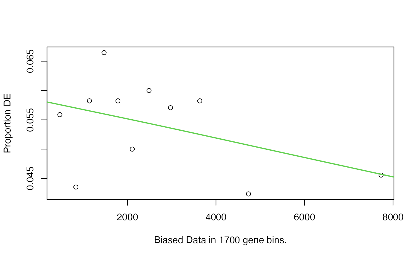
Then use goseq() function to perform the test by correcting the “gene length bias”:

tb1 = goseq(pwf, "hg19", "ensGene")
head(tb1)

##        category over_represented_pvalue under_represented_pvalue numDEInCat
## 3416 GO:0006955            1.807200e-64                        1        301
## 975  GO:0002376            8.377207e-59                        1        356
## 6472 GO:0019814            2.689698e-47                        1         70
## 3413 GO:0006952            1.012456e-46                        1        250
## 886  GO:0002250            7.007878e-42                        1        142
## 2571 GO:0005576            4.121990e-41                        1        396
##      numInCat                     term ontology
## 3416     1847          immune response       BP
## 975      2589    immune system process       BP
## 6472      138   immunoglobulin complex       CC
## 3413     1648         defense response       BP
## 886       662 adaptive immune response       BP
## 2571     3591     extracellular region       CC

Keep all genes

This time we keep the genes with p-values as NA (they are basically genes not expressed). We simply assume they are not DE.

tb = readRDS(system.file("extdata", "de.rds", package = "GSEAtraining"))
tb = tb[tb$symbol != "", ]  # keep pc genes

tb$fdr = p.adjust(tb$p_value, "BH")
genes = ifelse(tb$fdr < 0.05, 1, 0)
genes[is.na(genes)] = 0
names(genes) = tb$ensembl
table(genes)

## genes
##     0     1 
## 38668  1072

Let’s check the “bias distribution” again.

pwf = nullp(genes, "hg19", "ensGene")

## Loading hg19 length data...

## Warning in pcls(G): initial point very close to some inequality constraints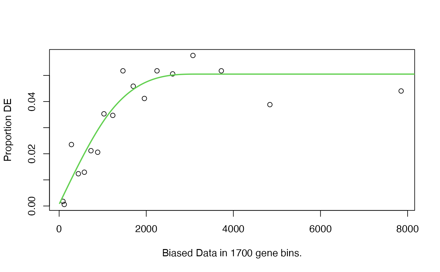

This becomes interesting. It shows a reverse pattern as in the original paper.

Note many lowly-expressed genes are short, so the increasing trend in the left part of the curve is from the proportion of “expressed genes” getting higher? Or can we say actually there is no such bias as mentioned in the goseq paper?

We perform the test:

tb2 = goseq(pwf, "hg19", "ensGene")

Compare tb1 and tb2

We compare tb1 and tb2:

library(eulerr)
lt = list(
    test1 = tb1$category[p.adjust(tb1$over_represented_pvalue, "BH") < 0.05], 
    test2 = tb2$category[p.adjust(tb2$over_represented_pvalue, "BH") < 0.05]
)
plot(euler(lt), quantities = TRUE)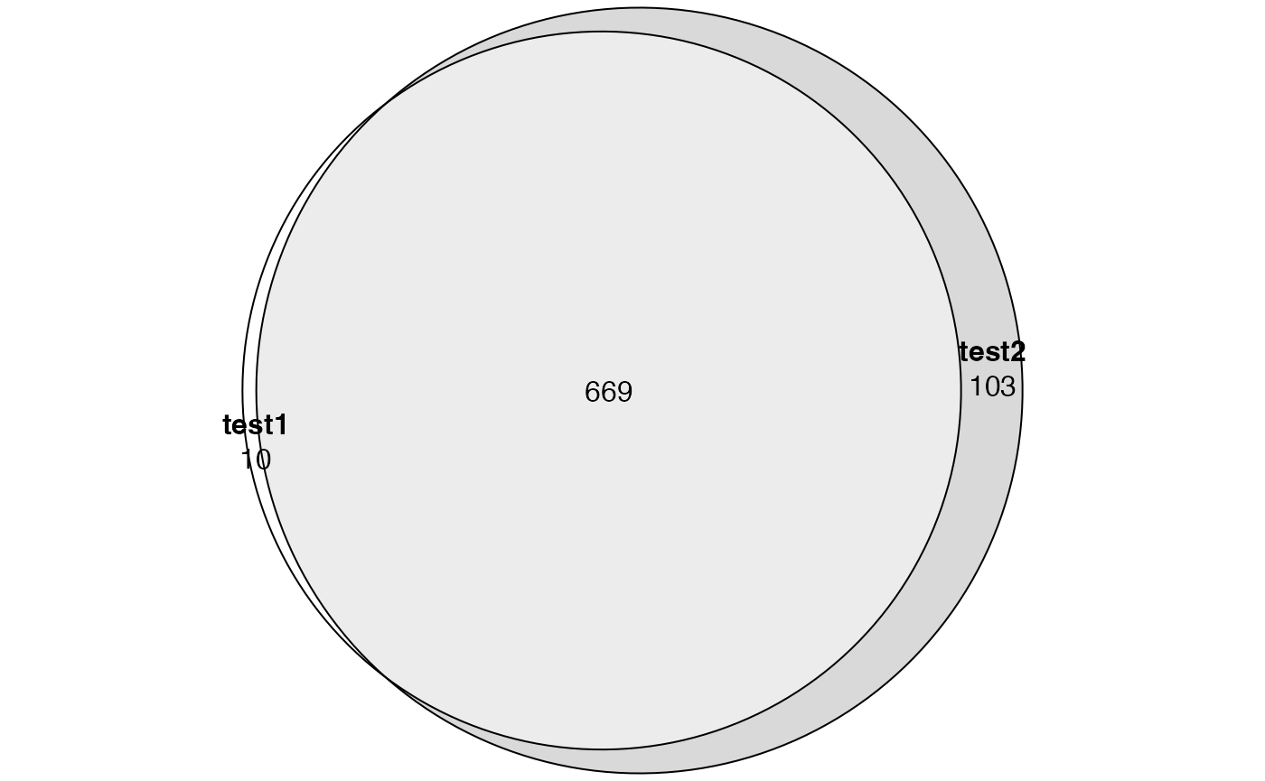

Does it mean the correction has no effect?

Compare to ORA

We also compare to ORA.

l = tb$fdr < 0.05; l[is.na(l)] = FALSE
diff_gene = tb$ensembl[l]

diff_gene are Ensembl IDs. We convert them to Entrez IDs:

library(GSEAtraining)
diff_gene = convert_to_entrez_id(diff_gene)

## 'select()' returned 1:many mapping between keys and columns

We use clusterProfiler to perform ORA analysis:

library(clusterProfiler)
library(org.Hs.eg.db)
tb3 = enrichGO(gene = diff_gene, ont = "BP", OrgDb = org.Hs.eg.db)

Now we compare ORA to GOseq results. Note tb1 and tb2 contains results for all three ontologies (BP, CC, MF). Here we only need BP.

tb1 = tb1[tb1$ontology == "BP", ]
tb2 = tb2[tb2$ontology == "BP", ]

library(eulerr)
lt = list(
    test1 = tb1$category[p.adjust(tb1$over_represented_pvalue, "BH") < 0.05], 
    test2 = tb2$category[p.adjust(tb2$over_represented_pvalue, "BH") < 0.05],
    ora = tb3$ID[p.adjust(tb3$pvalue, "BH") < 0.05]
)
plot(euler(lt), quantities = TRUE)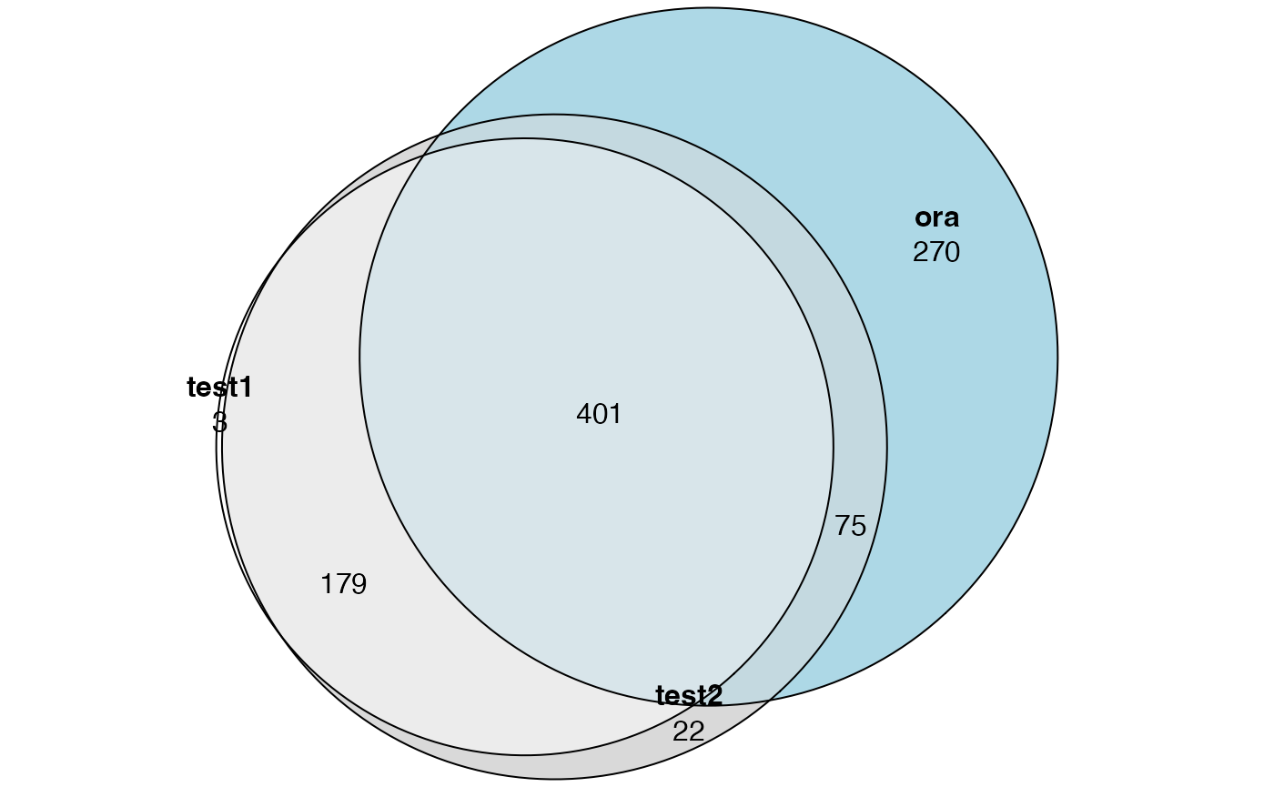

Conclusion: goseq was designed when the Possion distribution was used for DE analysis and maybe it does not help nowadays when more advanced DE methods are used.