Topic 2-02: Implement ORA from stratch
Zuguang Gu z.gu@dkfz.de
2025-03-02
Source:vignettes/topic2_02_implement_ora.Rmd
topic2_02_implement_ora.RmdImplementing ORA is very simple. As long as genes and gene sets are already in the correct ID types and formats, the implementation of ORA only needs several lines.
Three inputs for ORA:
- a vector of (DE) genes:
genes - a list of vectors where each vector contains genes in a gene set:
gene_sets - a vector of background genes:
universe
We calculate the following numbers:
Number of total genes:
n_universe = length(universe)Number of DE genes:
n_genes = length(genes)Sizes of gene sets:
m = sapply(gene_sets, length)Number of DE genes in gene sets:
We rename n_genes to k:
k = n_genesWe put these variables into the 2x2 contigency table:
| in the set | not in the set | total | |
|---|---|---|---|
| DE | x |
- | k |
| not DE | - | - | - |
| total | m |
- | n_universe |
Then we can calculate p-values from the hypergeometric distribution as:
phyper(x - 1, m, n_universe - m, k, lower.tail = FALSE)which is the same as:
phyper(x - 1, k, n_universe - k, m, lower.tail = FALSE)Let’s put all these code into a function:
ora = function(genes, gene_sets, universe) {
    n_universe = length(universe)
    n_genes = length(genes)

    x = sapply(gene_sets, function(x) length(intersect(x, genes)))
    m = sapply(gene_sets, length)
    n = n_universe - m
    k = n_genes

    p = phyper(x - 1, m, n, k, lower.tail = FALSE)

    data.frame(
        gene_set = names(gene_sets),
        hits = x,
        n_genes = k,
        n_gs = m,
        n_total = n_universe,
        p_value = p
    )
}
We can further improve the function by:
- set the default of
universeto the total genes ingene_sets - intersect
genesandgene_setstouniverse. Note this step also removes duplicated genes - add adjusted log2 fold enrichment and p-values
- order the result table by the significance
ora = function(genes, gene_sets, universe = NULL) {

    if(is.null(universe)) {
        universe = unique(unlist(gene_sets))
    } else {
        universe = unique(universe)
    }
    # restrict in universe
    genes = intersect(genes, universe)
    gene_sets = lapply(gene_sets, function(x) intersect(x, universe))

    n_universe = length(universe)
    n_genes = length(genes)

    x = sapply(gene_sets, function(x) length(intersect(x, genes)))
    m = sapply(gene_sets, length)
    n = n_universe - m
    k = n_genes

    p = phyper(x - 1, m, n, k, lower.tail = FALSE)

    df = data.frame(
        gene_set = names(gene_sets),
        hits = x,
        n_genes = k,
        n_gs = m,
        n_total = n_universe,
        log2fe = log2(x*n_universe/k/m),
        p_value = p
    )

    df$p_adjust = p.adjust(df$p_value, "BH")
    rownames(df) = df$gene_set
    df[order(df$p_adjust, df$p_value), ,drop = FALSE]
}
Let’s try our ora() with 1000 random genes on the MSigDB hallmark gene sets. get_msigdb() is from the GSEAtraining package.
library(org.Hs.eg.db)## Loading required package: AnnotationDbi## Loading required package: stats4## Loading required package: BiocGenerics##
## Attaching package: 'BiocGenerics'## The following objects are masked from 'package:stats':
##
## IQR, mad, sd, var, xtabs## The following objects are masked from 'package:base':
##
## anyDuplicated, aperm, append, as.data.frame, basename, cbind,
## colnames, dirname, do.call, duplicated, eval, evalq, Filter, Find,
## get, grep, grepl, intersect, is.unsorted, lapply, Map, mapply,
## match, mget, order, paste, pmax, pmax.int, pmin, pmin.int,
## Position, rank, rbind, Reduce, rownames, sapply, saveRDS, setdiff,
## table, tapply, union, unique, unsplit, which.max, which.min## Loading required package: Biobase## Welcome to Bioconductor
##
## Vignettes contain introductory material; view with
## 'browseVignettes()'. To cite Bioconductor, see
## 'citation("Biobase")', and for packages 'citation("pkgname")'.## Loading required package: IRanges## Loading required package: S4Vectors##
## Attaching package: 'S4Vectors'## The following object is masked from 'package:utils':
##
## findMatches## The following objects are masked from 'package:base':
##
## expand.grid, I, unname## ##
## Attaching package: 'GSEAtraining'## The following object is masked _by_ '.GlobalEnv':
##
## orags = get_msigdb(version = "2023.2.Hs", collection = "h.all")
genes = random_genes(org.Hs.eg.db, 1000, "ENTREZID")## 'select()' returned 1:many mapping between keys and columns## gene_set hits
## HALLMARK_INTERFERON_GAMMA_RESPONSE HALLMARK_INTERFERON_GAMMA_RESPONSE 14
## HALLMARK_ANGIOGENESIS HALLMARK_ANGIOGENESIS 4
## HALLMARK_FATTY_ACID_METABOLISM HALLMARK_FATTY_ACID_METABOLISM 11
## HALLMARK_WNT_BETA_CATENIN_SIGNALING HALLMARK_WNT_BETA_CATENIN_SIGNALING 4
## HALLMARK_DNA_REPAIR HALLMARK_DNA_REPAIR 10
## HALLMARK_INTERFERON_ALPHA_RESPONSE HALLMARK_INTERFERON_ALPHA_RESPONSE 7
## n_genes n_gs n_total log2fe p_value
## HALLMARK_INTERFERON_GAMMA_RESPONSE 198 200 4384 0.6321742 0.06623134
## HALLMARK_ANGIOGENESIS 198 36 4384 1.2987505 0.07709367
## HALLMARK_FATTY_ACID_METABOLISM 198 158 4384 0.6243263 0.09950431
## HALLMARK_WNT_BETA_CATENIN_SIGNALING 198 42 4384 1.0763580 0.11940149
## HALLMARK_DNA_REPAIR 198 150 4384 0.5617849 0.13874350
## HALLMARK_INTERFERON_ALPHA_RESPONSE 198 97 4384 0.6761175 0.14704944
## p_adjust
## HALLMARK_INTERFERON_GAMMA_RESPONSE 0.9596053
## HALLMARK_ANGIOGENESIS 0.9596053
## HALLMARK_FATTY_ACID_METABOLISM 0.9596053
## HALLMARK_WNT_BETA_CATENIN_SIGNALING 0.9596053
## HALLMARK_DNA_REPAIR 0.9596053
## HALLMARK_INTERFERON_ALPHA_RESPONSE 0.9596053The only restriction of ora() is the ID type for genes should be the same as in gene_sets.
Practice
Practice 1
The file de.rds contains results from a differential expression (DE) analysis.
de = readRDS(system.file("extdata", "de.rds", package = "GSEAtraining"))
de = de[, c("symbol", "p_value")]
de = de[!is.na(de$p_value), ]
head(de)
## symbol p_value
## 1 TSPAN6 0.0081373337
## 2 TNMD 0.0085126916
## 3 DPM1 0.9874656931
## 4 SCYL3 0.2401551938
## 5 C1orf112 0.8884603214
## 6 FGR 0.0006134791Take the symbol and p_value columns, set cutoff of p_value to 0.05, 0.01 and 0.001 respectively to filter the significant DE genes (of course, in applications, you need to correct p-values), apply ora() to the three DE gene lists using the GO BP gene sets (think how to obtain the GO gene sets from org.Hs.eg.db) and compare the ORA results (the whatever comparison you can think of).
If you EntreZ ID in the gene sets, you need to convert gene symbols for the DE genes to EntreZ IDs. But you can also choose to use gene symbols in the gene sets.
Solution
The three DE gene lists:
de_genes_1 = de$symbol[de$p_value < 0.05]
de_genes_2 = de$symbol[de$p_value < 0.01]
de_genes_3 = de$symbol[de$p_value < 0.001]

length(de_genes_1)
## [1] 3156length(de_genes_2)## [1] 1708length(de_genes_3)## [1] 817Get the GO BP gene sets. Note genes in de_genes_* are symbols, thus genes in gene sets should also be symbols.
gs = get_GO_gene_sets_from_orgdb(org.Hs.eg.db, "BP", gene_id_type = "SYMBOL")## 'select()' returned 1:many mapping between keys and columnsgs[1]## $`GO:0000002`
## [1] "PARP1" "SLC25A4" "DNA2" "TYMP" "ENDOG" "LIG3"
## [7] "MEF2A" "MPV17" "OPA1" "POLG" "RRM1" "SSBP1"
## [13] "TOP3A" "TP53" "DNAJA3" "LONP1" "AKT3" "POLG2"
## [19] "RRM2B" "SLC25A36" "TWNK" "METTL4" "PIF1" "SESN2"
## [25] "SLC25A33" "NEURL4" "MGME1" "CHCHD4" "PRIMPOL" "STOX1"We perform ORA for the three DE gene lists.
Compare number of significant GO terms:
sum(tb1$p_adjust < 0.05)## [1] 1023sum(tb2$p_adjust < 0.05)## [1] 866sum(tb3$p_adjust < 0.05)## [1] 752Actually we can see gene set enrichment analysis is a very robust method which is not sensitive to DE cutoffs (at least for this dataset).
Make a Venn (Euler) diagram:
library(eulerr)
plot(euler(list("DE_cutoff_0.05"  = tb1$gene_set[tb1$p_adjust < 0.05],
                "DE_cutoff_0.01"  = tb2$gene_set[tb2$p_adjust < 0.05],
                "DE_cutoff_0.001" = tb3$gene_set[tb3$p_adjust < 0.05])),
     quantities = TRUE)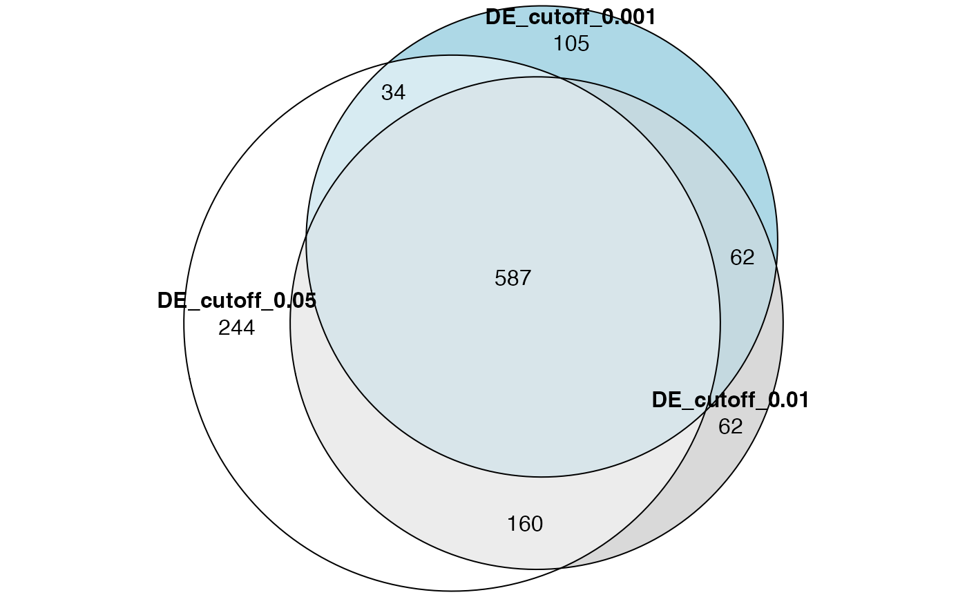
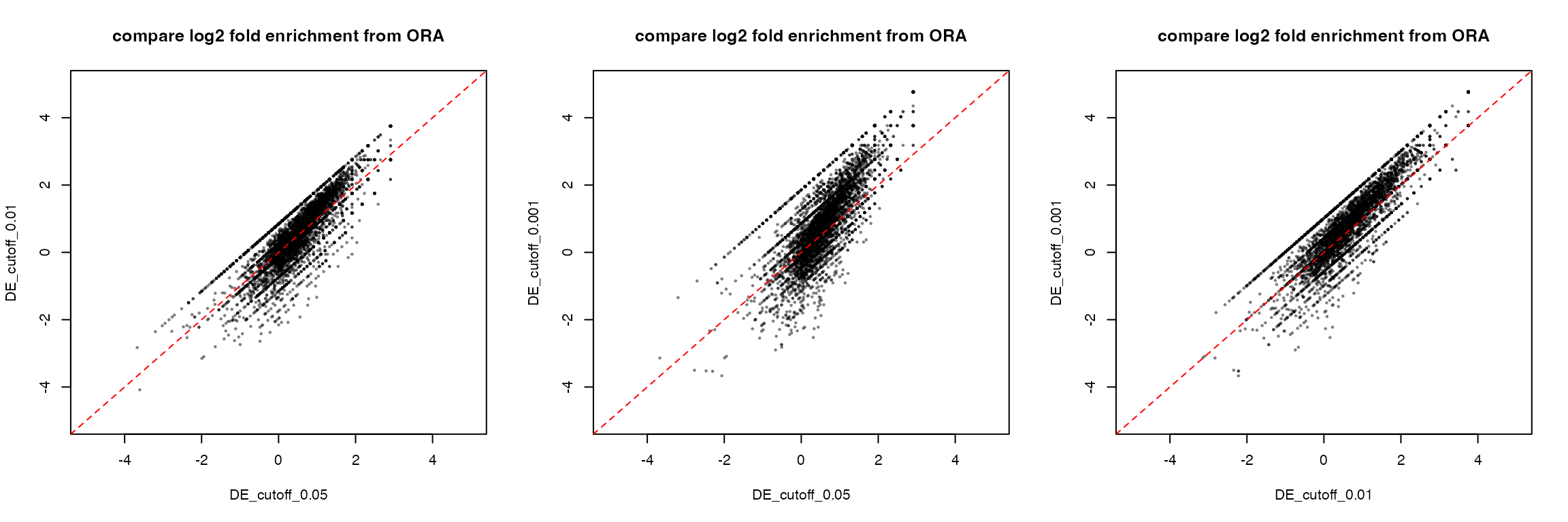
Compare log2 fold enrichment from the three ORA results. First take the common GO terms in the three ORA tables.
Then simply make pairwise scatter plots:
par(mfrow = c(1, 3))
plot(tb1[cn, "log2fe"], tb2[cn, "log2fe"], pch = 16, cex = 0.5, col = "#00000080",
    xlim = c(-5, 5), ylim = c(-5, 5), main = "compare log2 fold enrichment from ORA",
    xlab = "DE_cutoff_0.05", ylab = "DE_cutoff_0.01")
abline(a = 0, b = 1, lty = 2, col = "red")

plot(tb1[cn, "log2fe"], tb3[cn, "log2fe"], pch = 16, cex = 0.5, col = "#00000080",
    xlim = c(-5, 5), ylim = c(-5, 5), main = "compare log2 fold enrichment from ORA",
    xlab = "DE_cutoff_0.05", ylab = "DE_cutoff_0.001")
abline(a = 0, b = 1, lty = 2, col = "red")

plot(tb2[cn, "log2fe"], tb3[cn, "log2fe"], pch = 16, cex = 0.5, col = "#00000080",
    xlim = c(-5, 5), ylim = c(-5, 5), main = "compare log2 fold enrichment from ORA",
    xlab = "DE_cutoff_0.01", ylab = "DE_cutoff_0.001")
abline(a = 0, b = 1, lty = 2, col = "red")