Topic 5-01: Similarities of terms

There are two types of methods to calculate similarities between functional terms.

purely based on the number of member genes.
based on the topology of the ontology.

We demonstrate it with significant terms from an ORA analysis.

library(GSEAtraining)
lt = readRDS(system.file("extdata", "ora.rds", package = "GSEAtraining"))
diff_gene = lt$diff_gene
diff_gene = convert_to_entrez_id(diff_gene)

##

##   gene id might be SYMBOL (p =  0.980 )

## 'select()' returned 1:many mapping between keys and columns

Similarity based on gene counts

First we use a small collection of gene sets, the KEGG pathways.

df = read.table(url("https://rest.kegg.jp/link/pathway/hsa"), sep = "\t")
df[, 1] = gsub("hsa:", "", df[, 1])
df[, 2] = gsub("path:",  "", df[, 2])
head(df)

##      V1       V2
## 1 10327 hsa00010
## 2   124 hsa00010
## 3   125 hsa00010
## 4   126 hsa00010
## 5   127 hsa00010
## 6   128 hsa00010

We also retrieve the pathway names.

pathway_names = read.table(url("https://rest.kegg.jp/list/pathway/hsa"), sep = "\t")
pathway_names = structure(gsub(" - Homo .*$", "", pathway_names[, 2]), names = pathway_names[, 1])

Perform ORA analysis with clusterProfiler. There are 33 significant pathways.

library(clusterProfiler)

##

## Registered S3 methods overwritten by 'treeio':
##   method              from    
##   MRCA.phylo          tidytree
##   MRCA.treedata       tidytree
##   Nnode.treedata      tidytree
##   Ntip.treedata       tidytree
##   ancestor.phylo      tidytree
##   ancestor.treedata   tidytree
##   child.phylo         tidytree
##   child.treedata      tidytree
##   full_join.phylo     tidytree
##   full_join.treedata  tidytree
##   groupClade.phylo    tidytree
##   groupClade.treedata tidytree
##   groupOTU.phylo      tidytree
##   groupOTU.treedata   tidytree
##   inner_join.phylo    tidytree
##   inner_join.treedata tidytree
##   is.rooted.treedata  tidytree
##   nodeid.phylo        tidytree
##   nodeid.treedata     tidytree
##   nodelab.phylo       tidytree
##   nodelab.treedata    tidytree
##   offspring.phylo     tidytree
##   offspring.treedata  tidytree
##   parent.phylo        tidytree
##   parent.treedata     tidytree
##   root.treedata       tidytree
##   rootnode.phylo      tidytree
##   sibling.phylo       tidytree

## clusterProfiler v4.8.3  For help: https://yulab-smu.top/biomedical-knowledge-mining-book/
## 
## If you use clusterProfiler in published research, please cite:
## T Wu, E Hu, S Xu, M Chen, P Guo, Z Dai, T Feng, L Zhou, W Tang, L Zhan, X Fu, S Liu, X Bo, and G Yu. clusterProfiler 4.0: A universal enrichment tool for interpreting omics data. The Innovation. 2021, 2(3):100141

## 
## Attaching package: 'clusterProfiler'

## The following object is masked from 'package:stats':
## 
##     filter

tb = enricher(diff_gene, TERM2GENE = df[, 2:1])
sig_pathways = as.data.frame(tb)$ID

gs_pathway = split(df[, 1], df[, 2])
gs_pathway = gs_pathway[sig_pathways]

There are four similarity methods which are based on the counts:

Jaccard coeffcient
Dice coeffcient
Overlap coeffcient
Kappa coeffcient

Since Dice coeffcient is just a simple transformation from the Jaccard coeffcient, we only look at the following three methods:

library(simplifyEnrichment)

## Loading required package: BiocGenerics

## 
## Attaching package: 'BiocGenerics'

## The following objects are masked from 'package:stats':
## 
##     IQR, mad, sd, var, xtabs

## The following objects are masked from 'package:base':
## 
##     Filter, Find, Map, Position, Reduce, anyDuplicated, aperm, append,
##     as.data.frame, basename, cbind, colnames, dirname, do.call,
##     duplicated, eval, evalq, get, grep, grepl, intersect, is.unsorted,
##     lapply, mapply, match, mget, order, paste, pmax, pmax.int, pmin,
##     pmin.int, rank, rbind, rownames, sapply, setdiff, sort, table,
##     tapply, union, unique, unsplit, which.max, which.min

## Loading required package: grid

## ========================================
## simplifyEnrichment version 1.11.1
## Bioconductor page: https://bioconductor.org/packages/simplifyEnrichment/
## Github page: https://github.com/jokergoo/simplifyEnrichment
## Documentation: https://jokergoo.github.io/simplifyEnrichment/
## Examples: https://simplifyenrichment.github.io/
## 
## If you use it in published research, please cite:
## Gu, Z. simplifyEnrichment: an R/Bioconductor package for Clustering and 
##   Visualizing Functional Enrichment Results, Genomics, Proteomics & 
##   Bioinformatics 2022.
## 
## This message can be suppressed by:
##   suppressPackageStartupMessages(library(simplifyEnrichment))
## ========================================

m1 = term_similarity(gs_pathway, method = "jaccard")
m2 = term_similarity(gs_pathway, method = "overlap")
m3 = term_similarity(gs_pathway, method = "kappa")

Values on diagonals of the three symmetric matrices are 1. Since other values in the matrices are much smaller than 1, we set the diagonals to NA to improve the heatmap visualization.

diag(m1) = NA
diag(m2) = NA
diag(m3) = NA

library(ComplexHeatmap)

## ========================================
## ComplexHeatmap version 2.18.0
## Bioconductor page: http://bioconductor.org/packages/ComplexHeatmap/
## Github page: https://github.com/jokergoo/ComplexHeatmap
## Documentation: http://jokergoo.github.io/ComplexHeatmap-reference
## 
## If you use it in published research, please cite either one:
## - Gu, Z. Complex Heatmap Visualization. iMeta 2022.
## - Gu, Z. Complex heatmaps reveal patterns and correlations in multidimensional 
##     genomic data. Bioinformatics 2016.
## 
## 
## The new InteractiveComplexHeatmap package can directly export static 
## complex heatmaps into an interactive Shiny app with zero effort. Have a try!
## 
## This message can be suppressed by:
##   suppressPackageStartupMessages(library(ComplexHeatmap))
## ========================================

Heatmap(m1, name = "jaccard") + 
    rowAnnotation(pathway_name = anno_text(pathway_names[rownames(m1)]))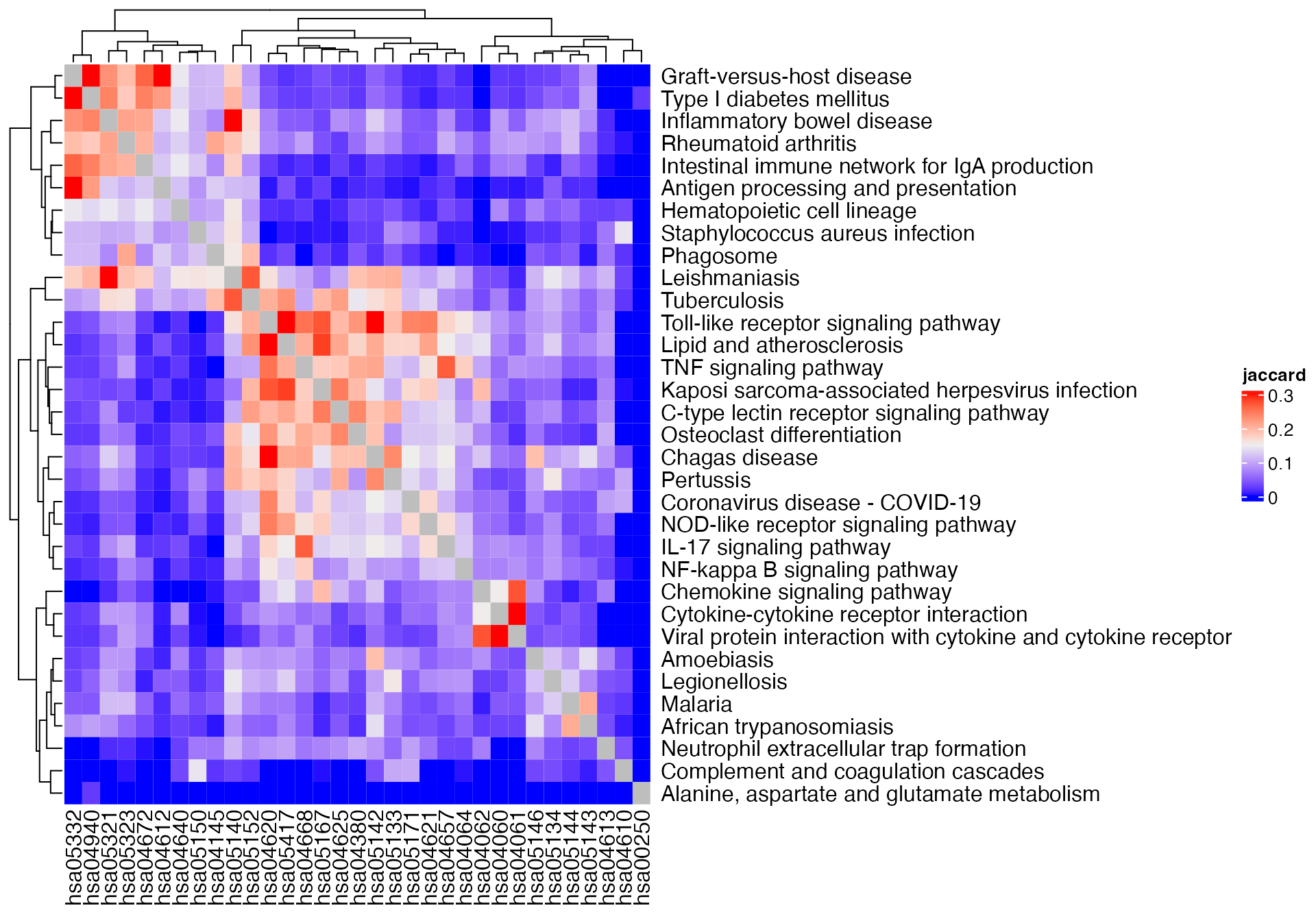

Heatmap(m2, name = "overlap") + 
    rowAnnotation(pathway_name = anno_text(pathway_names[rownames(m1)]))

Heatmap(m3, name = "kappa") + 
    rowAnnotation(pathway_name = anno_text(pathway_names[rownames(m1)]))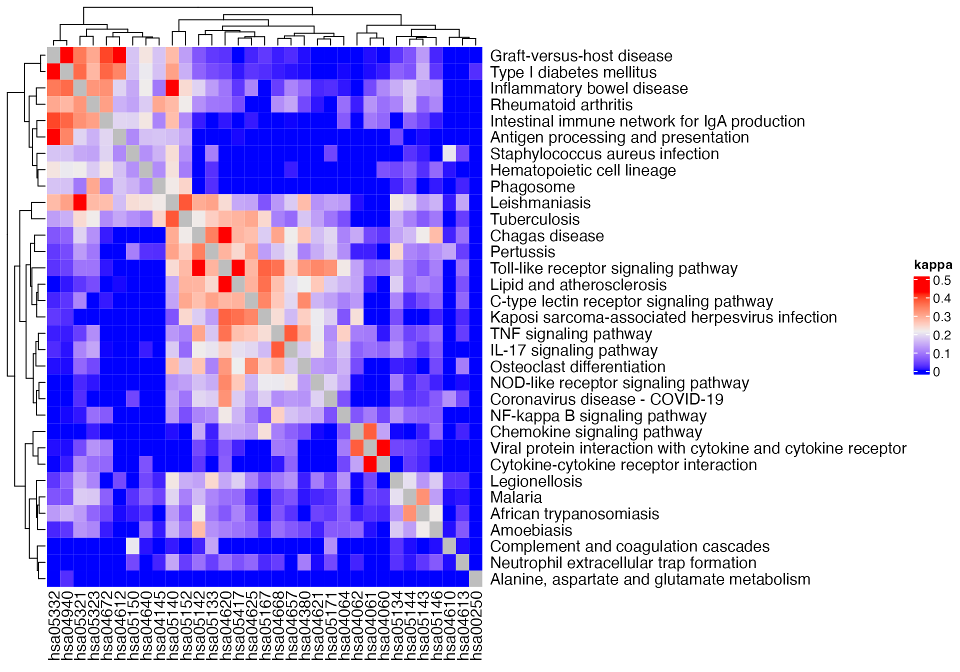

In previous examples, we use all genes in the gene sets. Next we restrict only to the DE genes.

m1 = term_similarity(gs_pathway, method = "jaccard", all = diff_gene)
m2 = term_similarity(gs_pathway, method = "overlap", all = diff_gene)
m3 = term_similarity(gs_pathway, method = "kappa", all = diff_gene)

diag(m1) = NA
diag(m2) = NA
diag(m3) = NA

Heatmap(m1, name = "jaccard") + 
    rowAnnotation(pathway_name = anno_text(pathway_names[rownames(m1)]))

## The automatically generated colors map from the 1^st and 99^th of the
## values in the matrix. There are outliers in the matrix whose patterns
## might be hidden by this color mapping. You can manually set the color
## to `col` argument.
## 
## Use `suppressMessages()` to turn off this message.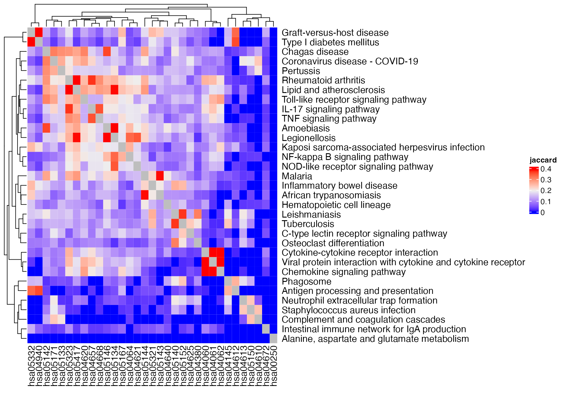

Heatmap(m2, name = "overlap") + 
    rowAnnotation(pathway_name = anno_text(pathway_names[rownames(m1)]))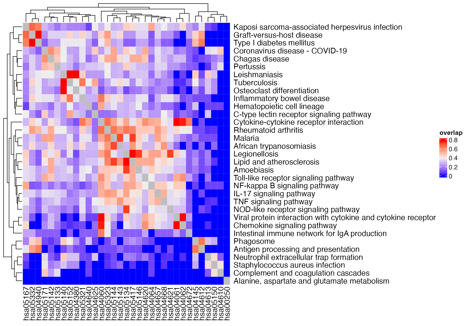

Heatmap(m3, name = "kappa") + 
    rowAnnotation(pathway_name = anno_text(pathway_names[rownames(m1)]))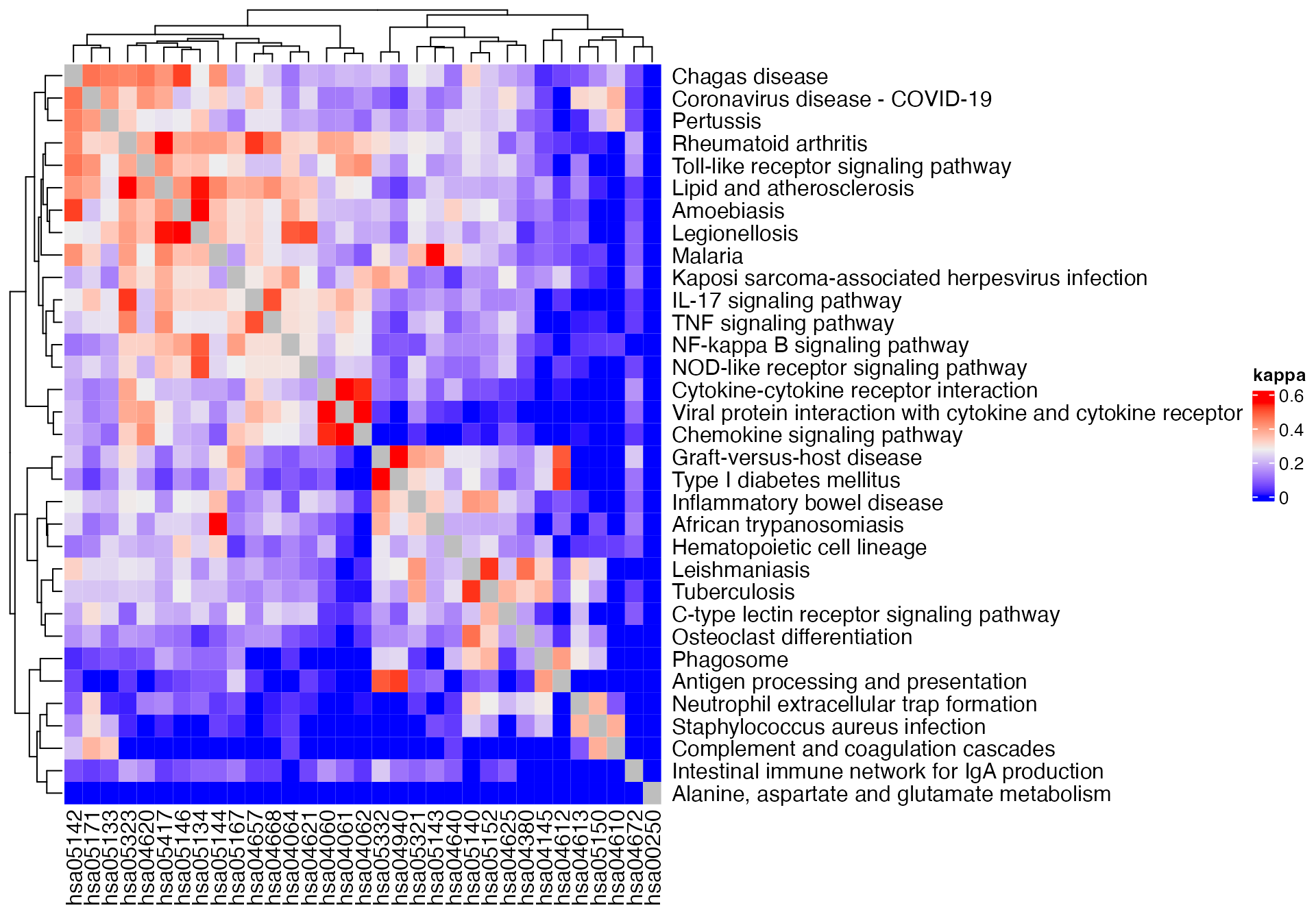

Next we use a much larger gene set collection: the GO gene sets:

library(org.Hs.eg.db)

## Loading required package: AnnotationDbi

## Loading required package: stats4

## Loading required package: Biobase

## Welcome to Bioconductor
## 
##     Vignettes contain introductory material; view with
##     'browseVignettes()'. To cite Bioconductor, see
##     'citation("Biobase")', and for packages 'citation("pkgname")'.

## Loading required package: IRanges

## Loading required package: S4Vectors

## Warning: package 'S4Vectors' was built under R version 4.3.2

## 
## Attaching package: 'S4Vectors'

## The following object is masked from 'package:clusterProfiler':
## 
##     rename

## The following object is masked from 'package:utils':
## 
##     findMatches

## The following objects are masked from 'package:base':
## 
##     I, expand.grid, unname

## 
## Attaching package: 'IRanges'

## The following object is masked from 'package:clusterProfiler':
## 
##     slice

## 
## Attaching package: 'AnnotationDbi'

## The following object is masked from 'package:clusterProfiler':
## 
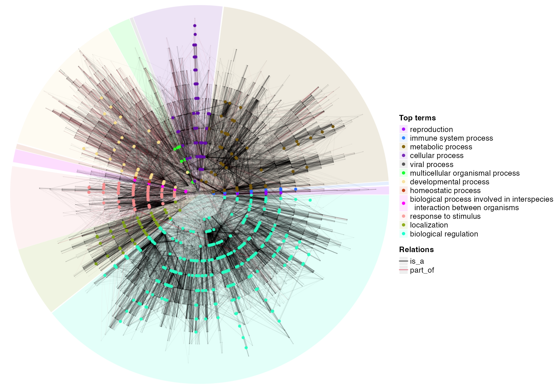
##     select

tb = enrichGO(gene = diff_gene, ont = "BP", OrgDb = org.Hs.eg.db)

sig_go = as.data.frame(tb)$ID

There are > 800 significant GO BP terms.

gs_bp = get_GO_gene_sets_from_orgdb(org.Hs.eg.db)

## 'select()' returned 1:many mapping between keys and columns

gs_bp = gs_bp[sig_go]

m1 = term_similarity(gs_bp, method = "jaccard")
m2 = term_similarity(gs_bp, method = "overlap")
m3 = term_similarity(gs_bp, method = "kappa")

diag(m1) = NA
diag(m2) = NA
diag(m3) = NA

Heatmap(m1, name = "jaccard", show_row_names = FALSE, show_column_names = FALSE,
    show_row_dend = FALSE, show_column_dend = FALSE)

## The automatically generated colors map from the 1^st and 99^th of the
## values in the matrix. There are outliers in the matrix whose patterns
## might be hidden by this color mapping. You can manually set the color
## to `col` argument.
## 
## Use `suppressMessages()` to turn off this message.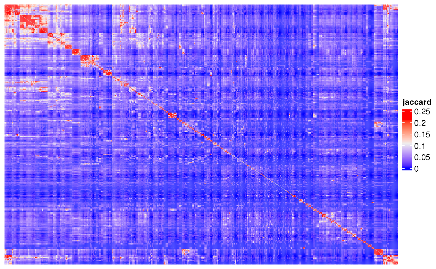

Heatmap(m2, name = "overlap", show_row_names = FALSE, show_column_names = FALSE,
    show_row_dend = FALSE, show_column_dend = FALSE)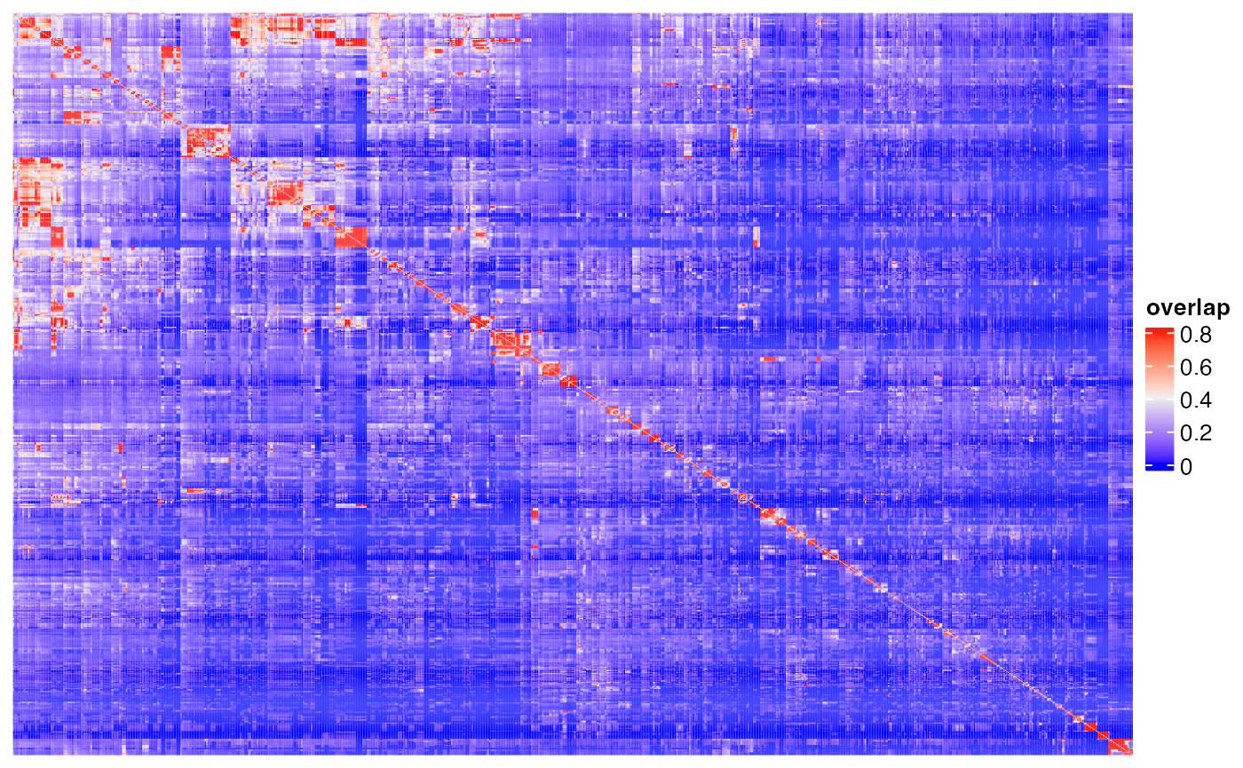

Heatmap(m3, name = "kappa", show_row_names = FALSE, show_column_names = FALSE,
    show_row_dend = FALSE, show_column_dend = FALSE)

## The automatically generated colors map from the 1^st and 99^th of the
## values in the matrix. There are outliers in the matrix whose patterns
## might be hidden by this color mapping. You can manually set the color
## to `col` argument.
## 
## Use `suppressMessages()` to turn off this message.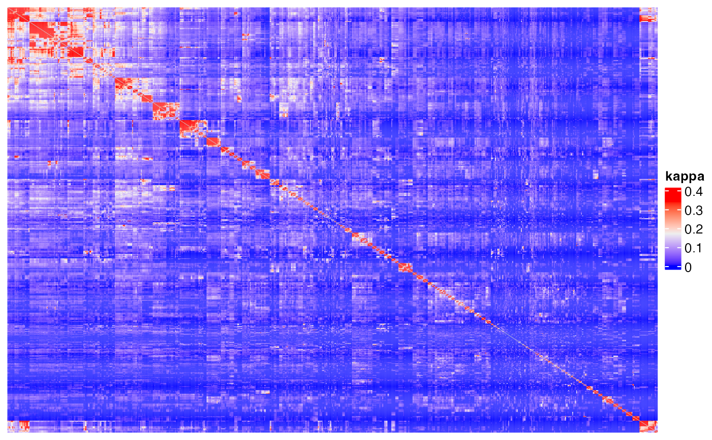

Or only restrict in DE genes

m1 = term_similarity(gs_bp, method = "jaccard", all = diff_gene)
m2 = term_similarity(gs_bp, method = "overlap", all = diff_gene)
m3 = term_similarity(gs_bp, method = "kappa", all = diff_gene)

diag(m1) = NA
diag(m2) = NA
diag(m3) = NA

Heatmap(m1, name = "jaccard", show_row_names = FALSE, show_column_names = FALSE,
    show_row_dend = FALSE, show_column_dend = FALSE)

## The automatically generated colors map from the 1^st and 99^th of the
## values in the matrix. There are outliers in the matrix whose patterns
## might be hidden by this color mapping. You can manually set the color
## to `col` argument.
## 
## Use `suppressMessages()` to turn off this message.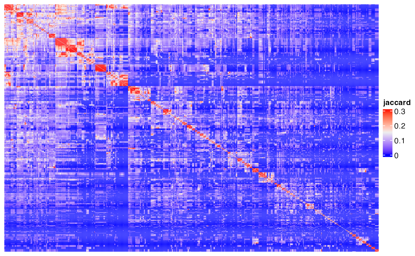

Heatmap(m2, name = "overlap", show_row_names = FALSE, show_column_names = FALSE,
    show_row_dend = FALSE, show_column_dend = FALSE)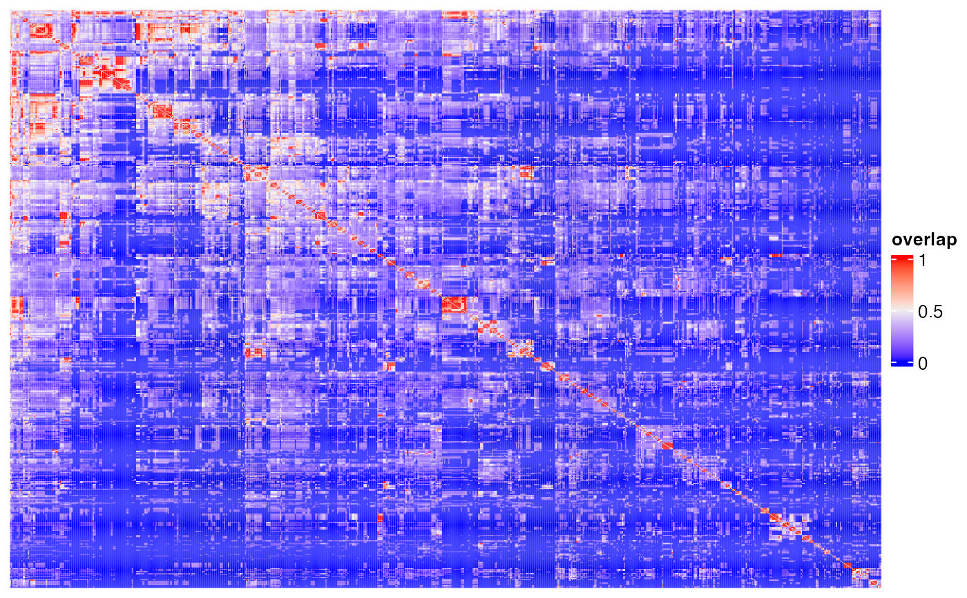

Heatmap(m3, name = "kappa", show_row_names = FALSE, show_column_names = FALSE,
    show_row_dend = FALSE, show_column_dend = FALSE)

## The automatically generated colors map from the 1^st and 99^th of the
## values in the matrix. There are outliers in the matrix whose patterns
## might be hidden by this color mapping. You can manually set the color
## to `col` argument.
## 
## Use `suppressMessages()` to turn off this message.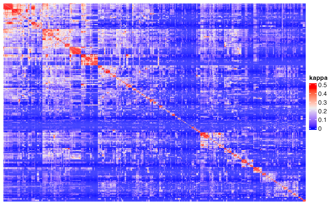

Semantic similarity based on ontology structures

There are also two major types of methods for semantic similarities.

based on external gene annotations
based on internal topology structure

Based on gene annotation

library(simona)
simona_opt$verbose = FALSE

dag = create_ontology_DAG_from_GO_db("BP", org_db = org.Hs.eg.db)

The Sim_Lin_1998 is one of the classic semantic similarity method.

m = term_sim(dag, sig_go, method = "Sim_Lin_1998")

## remove 16 terms with no annotation.

diag(m) = NA
Heatmap(m, name = "Sim_Lin_1998", show_row_names = FALSE, show_column_names = FALSE,
    show_row_dend = FALSE, show_column_dend = FALSE)

Purely based on the topology

The _Sim_WP_1994__ is one of the classic semantic similarity method.

m = term_sim(dag, sig_go, method = "Sim_WP_1994")
diag(m) = NA
Heatmap(m, name = "Sim_WP_1994", show_row_names = FALSE, show_column_names = FALSE,
    show_row_dend = FALSE, show_column_dend = FALSE)

Visualize the ontology

dag_circular_viz(dag, highlight = sig_go)

Zuguang Gu z.gu@dkfz.de

2024-01-26

Similarity based on gene counts

Semantic similarity based on ontology structures

Based on gene annotation

Purely based on the topology

Visualize the ontology